Some times we need to relearn the basics. Base (nucleotide) frequency per sequence (read) and positional frequency for each base are well understood at the time of first generation bioinformatics (with fasta sequences mostly). Now that are we into NGS, we forget (at least I) tend to forget the basics. For such people (like me), here is a  note on calculation base frequency per read and also positional frequency for a set of reads. Please note that tools such as FastQC does this. But FastQC does it for first few bases and there are several independent tools to do that.
For today, let us do this in R/Bioconductor. Packages used are biostrings for calculation and for  plotting, ggplot and reshape2 packages are used.
We can do this with both fastq and fasta files. For loading fasta files, code is at the end. For fastq and fasta code is same except for loading initial input files.
Let us take a fastq file with several reads. Each read has certain A, T, G, C and other bases (such as N, B etc). There are two cases here:
1) Let us say there are 20 reads and we want total number of As, Ts, Gs and Cs per read. We want it for all 20 reads.
2) Let us say there are 20 reads of length 55 nt. At each position of the read ( across 20 reads), we would like to have each base frequency or number i.e at position 1 of all 20 reads, how many As are there and how many Ts and how many Gs and so on.
Let us deal with first case. You can download example fastq file here. A little statistics about sample.fastq:
==============================================================
$ seqkit stats sample.fastq
file          format  type  num_seqs  sum_len  min_len  avg_len  max_len
sample.fastq  FASTQ   DNA         92   13,892      151      151      151
==============================================================
There are around 92 reads and average length of read is 151bp. Minimum and maximum length is 151 bp.
Let us do it using biostrings:
==============================================
# Load biostrings library
$ library(Biostrings)
# read fastq file into R and save it as object
$ fastq <- readDNAStringSet("sample.fastq","fastq")
# Now count the number of bases (ATGC and other) per each read and for all reads. #Number is expressed as percentage
$ freq <- alphabetFrequency(fastq, as.prob = T,baseOnly=T)
# Result is matrix. Now plot it using mat plot and type of graph is line graph
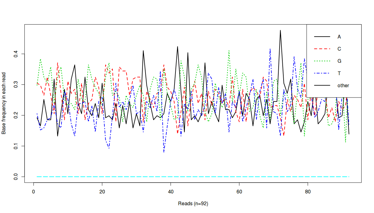
$ matplot(freq,type='l')
# Add legend to the image.
$ legend(legend = colnames(freq),"topright",lty=1:5,col=1:5)
=================================================
Final result:
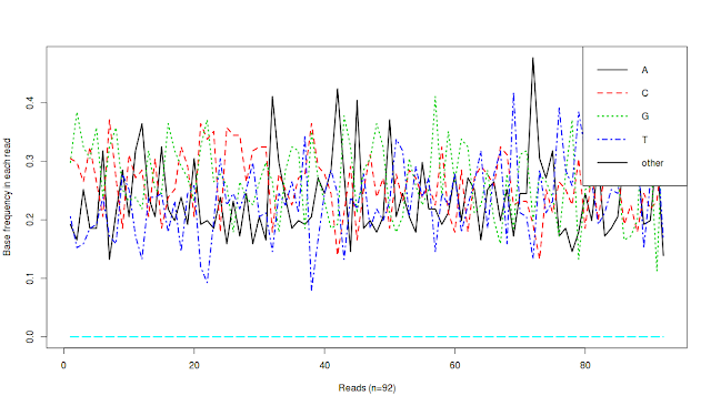What does this image tell us? It tells us that there are around ~90 sequences and in each sequence, we have percentage of each base (A, T, G, C and non-ATGC (other) bases)
Now let us address the second requirement where we need base frequency at each position, for all reads.
========================
## Load library
$ library(Biostrings)
## Read fastq file into R and save it as object
$ fastq <- readDNAStringSet("sample.fastq","fastq")
## Calculate base percentage at each position, for all reads
$ afmc=consensusMatrix(fastq, baseOnly=T,as.prob = T)
## Transpose the data frame
$ tafmc=t(afmc)
## Plot the data: -5 is to remove others column keeping only ATG and C columns
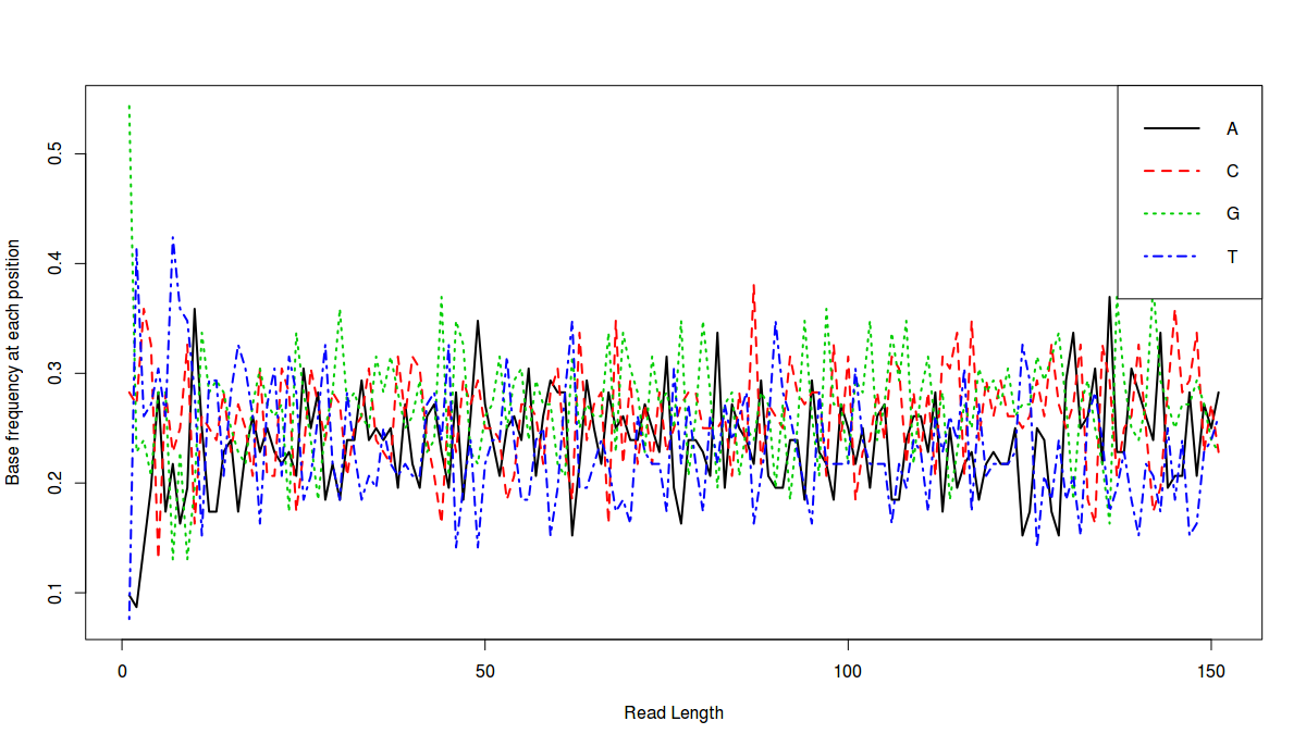
$ matplot(tafmc[,-5], type="l", lwd=2, xlab="Read Length", ylab= "Base frequency at each position")
## Add legend
$ legend(legend = colnames(tafmc)[-5],"topright",col=1:4, lty=1:4, lwd=2)
=====================================
Final result:
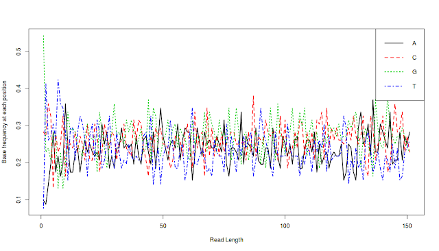What does this plot say. This plot says that the average length of all reads is a little more 150 bps and at each position (in all reads), we have percentage of each base, denoted by color lines.
Now can we draw in ggplot?
 =======================
## Load libraries ggplot2 and reshape2
$ library(ggplot2)
$ library(reshape2)
## Convert the data from wide format to long format
$ rtafmc=melt(tafmc)
## Now change the column names some meaning ful names
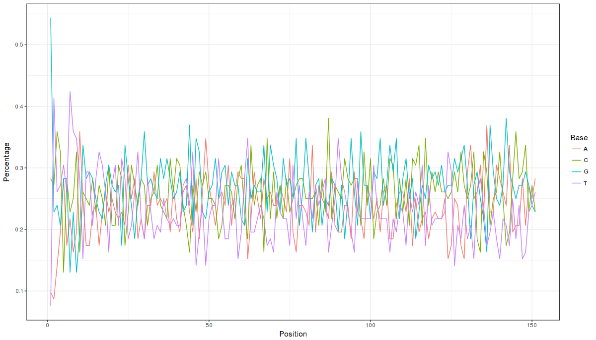
$ colnames(rtafmc)=c("Position","Base","Percentage")
## Let us draw and apply black and white theme instead of ggplot default theme. We want ##line plot and we would like only ATGC columns
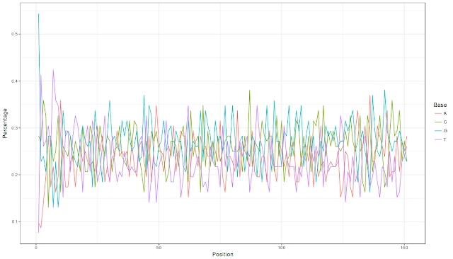
$ qplot(Position,Percentage, data=subset(rtafmc, Base!="other"), group=Base, geom="line", color=Base)+ theme_bw()
=======================
Let us look at the ggplot image (well, one can always improve the visualization:))

Now after doing this, one can always wonder about much easier way to do this. We have a library called SeqTools. Let us use that and see how easy it is:
===========================================
## Load SeqTools library
library(seqTools)
# Reads fastq file
fq=fastqq("sample.fastq")
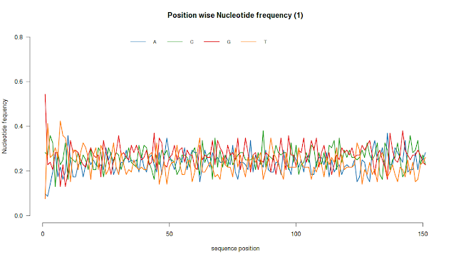
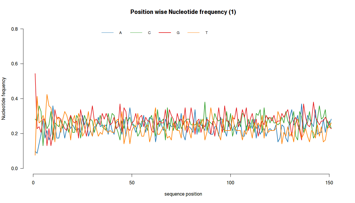
# Plots nucleotide frequency at each position
plotNucFreq(fq,1)
====================================