Parsing and annotation of statistically significant variants is very important in NGS analysis. Statistically variants are stored in standard format, well known as VCF. A variant of this format is called gVCF (genomic VCF) which stores base information at non-variant locations as well.
There are several public annotations available for variants identified in NGS studies. One of the best annotation is available as clinvar.vcf including curated polymorphic and clinically significant variants In this note, we use clinvar vcf and dplyr to extract information and we will use vcflib package to convert vcf to tab separated file.
In linux as well as windows, there are several good tools such as bcftools, vcflib to extract information from VCF. There are several tools available in R to manipulate VCF files using gRanges. However, we take an easy route in this note with following steps:
1) Download clinvar vcf file from NCBI or the example clinvar vcf ( ~ 6MB file and can be downloaded from here). (MD5sum: debad87790852ae518956ef0f3f3d453)
2) Convert clinvar vcf to tab separated file using vcf2tsv function available in package vcflib
3) Import tab separated file into R and analyze the data using dplyr.
Following commands are necessary for the steps mentioned above:
1) Download clinvar vcf (for hg38) from NCBI or from example clinvar.vcf link. ( 6MB file, MD5sum: debad87790852ae518956ef0f3f3d453)
2) Index gzipped VCF file. This would create a new file with ".tbi" extension which is index for the the vcf file.
command: tabix -p vcf <input.vcf>
Example: tabix -p vcf clinvar_GRCh38_12jul2015.vcf.gz
Please note that VCF file and index should be in the same directory for further processing and tabix program is part of vcflib
3) Convert vcf to tab separate values (tsv) file
command: vcf2tsv input.vcf.gz > output.tab
Example: vcf2tsv clinvar_GRCh38_12jul2015.vcf.gz > clinvar_GRCh38_12jul2015.vcf.tab
Cross checking VCF output:
1) Please note that ALT column in VCF file can have more than one allele. If there are more than one allele in ALT column, vcf2tsv creates row for each individual allele. Hence rows (records) in tab separated file must be more than vcf records.
2) In later steps, we are going to count single nt variations (SNVs), multi nt variations (MNV) and indels (DIVs). These must match with those from vcf statistics generated from bcf tools.
To generate vcf statistics, use following command:
command: bcftools stats input.vcf.gz > output.stats
ExampleL bcftools stats clinvar_GRCh38_12jul2015.vcf.gz > clinvar_GRCh38_12jul2015.vcf.stats
This would create a text file with total number of records, number of SNVs, MNVs, DIVs, transition/ transvertion ratio and other information related to VCF. we are going to match the numbers between output for dplyr and bcfstats, to cross check the output.
With clinvar.vcf in hand, we can ask several questions:
1) what is the most represented chromosome i.e chromosome with highest number of clinival variants?
2) What is the most represented diseases in clinivar.vcf?
3) What is the number of SNVs MNVs and DIVs in clinvar?
4) Which gene has highest number of variants ?
5) List of all variants sorted by genes (in decreasing order)..like wise.
We will try to answer few questions here with code. Rest questions (the ones you have) can be answered by adapting the code given below.
1) Before that let us load the tab separated values in R.
code: clinvar=read.delim2("input.tab", header=TRUE, sep="\t")
Example: clinvar=read.delim2("clinvar_GRCh38_12jul2015.vcf.tab", header=TRUE, sep="\t")
2) Let us check if all the entries are imported comparing lines (records) in input file and clinvar object in R.
code: dim(clinvar) # prints the length and variables in the clinvar. Please note down the length of the object.
In linux, open a terminal and type the following command:
code: wc -l <input.tab> # This would print total number of records in the input file.
Example: wc -l clinvar_GRCh38_12jul2015.vcf.tab
Compare the numbers. Since original file has headers, the two numbers differ by one header line ( for eg. 134207 in linux Vs 134206 in R).
3) One can also compare the headers of the file and column names of R object. Code is given below
Command in R: colnames(clinvar)
Header in linux: head -1 <input.tab>
Example in linux: head -1 clinvar_GRCh38_12jul2015.vcf.tab
Compare the two outputs, should be identical.
4) Load the following libraries, which we will be using in analysis and graphing
Command:
lib.pac= c("dplyr", "ggplot2", "ggvis")
lapply (lib.pac, require, character.only=TRUE)
This code would load all the 3 packages at the same time. If they do not exist, please install them. Arguments (commands) for dplyr will follow a logic outlined below:
data.frame <then> execute the commands <then> execute the commands <then> execute the commands. "then" is represented by "%>%"
5) List variants per chromosome (all SNVs, DIVs, MNVs together per chromosome)
Command: total.var.per.chr=clinvar %>% group_by(CHROM) %>% summarise(n=n())
6) View the first five lines
Command: head(total.var.per.chr)
These lines would give total number of variants per chromosome. Please note that chromosomes are not ordered alpha numerically/naturally/human sorted.
7) List all variants per each category of variants
Command: var.cat=clinvar %>% group_by(VC) %>% summarise(Variants=n())
View all variants per variant category
Command: var.cat
7) List variant categories per chromosome i.e list SNVs, DIVs and MNVs separately for each chromosome
Command: var.per.chr=clinvar %>% group_by(CHROM,VC) %>% summarise(n=n())
8) Print the first few lines of var.per.chr
Command: head (var.per.chr)
Lines would list SNVs, MNVs, DIVs individuall for each chromosome.
9) List only SNVs. Please note that this command can be adapted for DIVs and MNVs as well.
Command: clinvar.snv=clinvar %>% filter(VC=="SNV") %>% group_by(CHROM,VC) %>% summarise(n=n())
Please note that we are filtering column "VC" by "SNV". We can combine multiple terms here.
10) View the first few lines
Command: head(clinvar.snv)
11) Visualize the variants per chromosome. Please note that MNVs are very few compared to other categories. So one cannot visualize them without transforming the number of variants. Below, are two graphs : one with original numbers, the other with log (10) transformed values. We will be using ggvis for visualization. We can also use ggplot2. Code for ggplot2 is given at the end of the note.

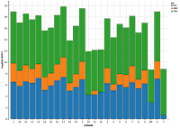 Figure a and b (please click to enlarge): Figure a without transformation and figure b with log(10) transformation.
Code:
Figure a: var.per.chr %>% ggvis (~CHROM,~Variants, fill=~VC) %>% layer_bars()
Figure b: var.per.chr %>% ggvis (~CHROM,~log(Variants), fill=~VC) %>% layer_bars()
In this figure, each bar is filled with colors as per variant category.
12) List top 5 genes with highest number of variants
Code: clinvar %>% filter (GENEINFO!=" ") %>% group_by (GENEINFO) %>% summarise (Variants=n()) %>% arrange(desc(Variants)) %>% slice(1:5)
logic: load data.frame clinvar <then> filter GENEINFO (gene symbol) column with no entries <then> group variants by gene symbol <then> count all the variants per gene and put in a new column titled "Variants" <then> arrange the genes by the number of variants per genes in descending order <then> display first 5 genes
13) List top 5 genes with highest number of SNVs. Please note that the command can be adapted to list genes with highest MNVs and DIVs.
Code: clinvar %>% filter (GENEINFO!="" & VC=="SNV") %>% group_by (GENEINFO) %>% summarise(Variants=n()) %>% arrange(desc(Variants)) %>% slice(1:5)
14) List the gene with highest number of variants
Code: clinvar%>% filter (GENEINFO !=" ") %>% group_by(GENEINFO) %>% summarise(n=n()) %>% filter (n==max(n))
15) List the gene with highest number of SNVs, MNVs and DIVs
Command for gene with highest number of
SNVs: clinvar%>% filter (GENEINFO !=" " & VC=="SNV") %>% group_by(GENEINFO) %>% summarise(n=n()) %>% filter (n==max(n))
MNVs: clinvar%>% filter (GENEINFO !=" " & VC=="MNV") %>% group_by(GENEINFO) %>% summarise(n=n()) %>% filter (n==max(n))
DIVs: clinvar%>% filter (GENEINFO !=" " & VC=="DIV") %>% group_by(GENEINFO) %>% summarise(n=n()) %>% filter (n==max(n))
16) Display gene with highest number of variants on each chromosome
Command: clinvar %>% group_by(CHROM,GENEINFO) %>% summarise(Genes=n()) %>% filter(Genes==max(Genes))
Please note that there are several entries in clinvar without gene name i.e variants might fall intergenic regions or gene deserts.
17) Display the chromosome with highest number of variants that fall in genes
Command: clinvar%>% filter (GENEINFO !=" ") %>% group_by(CHROM) %>% summarise(n=n()) %>% filter (n==max(n))
18) Display the chromosome with highest number of variants
Command: clinvar %>% group_by(CHROM) %>% summarise(n=n()) %>% filter (n==max(n))
19) Display the top 5 chromosomes with highest number of variants
Command: clinvar %>% group_by(CHROM) %>% summarise(Variants=n()) %>% arrange(desc(Variants)) %>% slice (1:5)
20) Display the top 5 genes with highest number of variants within each chromosome
Command: clinvar %>% filter (GENEINFO!=" ") %>% group_by(CHROM,GENEINFO) %>% summarise(variant=n()) %>% arrange(desc(variant)) %>% slice(1:5)
21) Display the top gene with highest number of variants within each chromosome
Command: clinvar %>% filter (GENEINFO!="") %>% group_by(CHROM,GENEINFO) %>% summarise(variant=n()) %>% filter(variant==max(variant))
22) Count and display variants for each gene
Command: clin.genes=clinvar%>% filter (GENEINFO !="") %>% group_by(GENEINFO) %>% summarise(count=n())
23) Display the first few lines
Command: head(clin.genes)
24) Display the number of genes on each chrosome in clinvar.vcf
Command: clinvar %>% select (CHROM, GENEINFO) %>% filter (GENEINFO != "") %>% distinct (GENEINFO) %>% group_by(CHROM) %>% summarise(Genes=n())
25) Display total number of genes in clinvar. vcf
Command: clinvar %>% select (CHROM, GENEINFO) %>% filter (GENEINFO != "") %>% distinct (GENEINFO) %>% summarise(Genes=n())
26) Display top 5 diseases on each chromosome i.e diseases with highest number of variants in both genic and intergenic regions
Command: clinvar %>% filter (CLNDBN!=" ") %>% group_by(CHROM,CLNDBN) %>% summarise(Variants=n()) %>% arrange(desc(Variants)) %>% slice(1:5)
27) List the disease category with highest number of variants
Command: clinvar %>% filter (CLNDBN!=" ") %>% group_by(CLNDBN) %>% summarise(Diseases=n()) %>% arrange(desc(Diseases)) %>% slice(1:5)
Total code:
# load tab file
clinvar=read.delim2("clinvar_GRCh38_12jul2015.vcf.tab", header=TRUE, sep="\t")
# dimensions of the file
dim(clinvar)
# headers of the file
colnames(clinvar)
# load libraries dplyr, ggvis, ggplot2
lib.pac= c("dplyr", "ggplot2", "ggvis")
lapply (lib.pac, require, character.only=TRUE)
# total variants per chromosome
total.var.per.chr=clinvar %>% group_by(CHROM) %>% summarise(n=n())
# total variant categories
var.cat=clinvar %>% group_by(VC) %>% summarise(Variants=n())
var.cat
# variant categories per chromosome
var.per.chr=clinvar %>% group_by(CHROM,VC) %>% summarise(n=n())
# Print only SNVs
clinvar.snv=clinvar %>% filter(VC=="SNV") %>% group_by(CHROM,VC) %>% summarise(n=n())
# Visualize categories per chromosome
var.per.chr %>% ggvis (~CHROM,~Variants, fill=~VC) %>% layer_bars()
var.per.chr %>% ggvis (~CHROM,~log(Variants), fill=~VC) %>% layer_bars()
# Top 5 genes with highest number of variants
clinvar %>% filter (GENEINFO!="") %>% group_by (GENEINFO) %>% summarise(Variants=n()) %>% arrange(desc(Variants)) %>% slice(1:5)
# Gene with highest number of variants
clinvar%>% filter (GENEINFO !="") %>% group_by(GENEINFO) %>% summarise(n=n()) %>% filter (n==max(n))
# Gene with highest number of SNVs
clinvar%>% filter (GENEINFO !="" & VC=="SNV") %>% group_by(GENEINFO) %>% summarise(n=n()) %>% filter (n==max(n))
# Gene with highest number of MNVs
clinvar%>% filter (GENEINFO !="" & VC=="MNV") %>% group_by(GENEINFO) %>% summarise(n=n()) %>% filter (n==max(n))
# Gene with highest number of DIVs
clinvar%>% filter (GENEINFO !="" & VC=="DIV") %>% group_by(GENEINFO) %>% summarise(n=n()) %>% filter (n==max(n))
# Display the chromsome with highest number of variants in gene regions
clinvar%>% filter (GENEINFO !="") %>% group_by(CHROM) %>% summarise(n=n()) %>% filter (n==max(n))
# Display the chromsome with highest number of variants
clinvar %>% group_by(CHROM) %>% summarise(n=n()) %>% filter (n==max(n))
# List top 5 chromosomes with highest number of variants
clinvar %>% group_by(CHROM) %>% summarise(Variants=n()) %>% arrange(desc(Variants)) %>% slice (1:5)
# Display the top 5 genes with highest variants per each chromosome
clinvar %>% filter (GENEINFO!="") %>% group_by(CHROM,GENEINFO) %>% summarise(variant=n()) %>% arrange(desc(variant)) %>% slice(1:5)
# Display the gene with highest variants per each chromosome
clinvar %>% filter (GENEINFO!="") %>% group_by(CHROM,GENEINFO) %>% summarise(variant=n()) %>% filter(variant==max(variant))
# Display number of variants per each gene
clin.genes=clinvar%>% filter (GENEINFO !="") %>% group_by(GENEINFO) %>% summarise(count=n())
head(clin.genes)
# Display the number of genes per chromosome
clinvar %>% select (CHROM, GENEINFO) %>% filter (GENEINFO != "") %>% distinct (GENEINFO) %>% group_by(CHROM) %>% summarise(Genes=n())
# total number of genes in clinvar
clinvar %>% select (CHROM, GENEINFO) %>% filter (GENEINFO != "") %>% distinct (GENEINFO) %>% summarise(Genes=n())
#total diseases per chromosome, sorted and top 5
clinvar %>% filter (CLNDBN!="") %>% group_by(CHROM,CLNDBN) %>% summarise(Diseases=n()) %>% arrange(desc(Diseases)) %>% slice(1:5)
#Top 5 diseases
clinvar %>% filter (CLNDBN!="") %>% group_by(CLNDBN) %>% summarise(Diseases=n()) %>% arrange(desc(Diseases)) %>% slice(1:5)
There are several public annotations available for variants identified in NGS studies. One of the best annotation is available as clinvar.vcf including curated polymorphic and clinically significant variants In this note, we use clinvar vcf and dplyr to extract information and we will use vcflib package to convert vcf to tab separated file.
In linux as well as windows, there are several good tools such as bcftools, vcflib to extract information from VCF. There are several tools available in R to manipulate VCF files using gRanges. However, we take an easy route in this note with following steps:
1) Download clinvar vcf file from NCBI or the example clinvar vcf ( ~ 6MB file and can be downloaded from here). (MD5sum: debad87790852ae518956ef0f3f3d453)
2) Convert clinvar vcf to tab separated file using vcf2tsv function available in package vcflib
3) Import tab separated file into R and analyze the data using dplyr.
Following commands are necessary for the steps mentioned above:
1) Download clinvar vcf (for hg38) from NCBI or from example clinvar.vcf link. ( 6MB file, MD5sum: debad87790852ae518956ef0f3f3d453)
2) Index gzipped VCF file. This would create a new file with ".tbi" extension which is index for the the vcf file.
command: tabix -p vcf <input.vcf>
Example: tabix -p vcf clinvar_GRCh38_12jul2015.vcf.gz
Please note that VCF file and index should be in the same directory for further processing and tabix program is part of vcflib
3) Convert vcf to tab separate values (tsv) file
command: vcf2tsv input.vcf.gz > output.tab
Example: vcf2tsv clinvar_GRCh38_12jul2015.vcf.gz > clinvar_GRCh38_12jul2015.vcf.tab
Cross checking VCF output:
1) Please note that ALT column in VCF file can have more than one allele. If there are more than one allele in ALT column, vcf2tsv creates row for each individual allele. Hence rows (records) in tab separated file must be more than vcf records.
2) In later steps, we are going to count single nt variations (SNVs), multi nt variations (MNV) and indels (DIVs). These must match with those from vcf statistics generated from bcf tools.
To generate vcf statistics, use following command:
command: bcftools stats input.vcf.gz > output.stats
ExampleL bcftools stats clinvar_GRCh38_12jul2015.vcf.gz > clinvar_GRCh38_12jul2015.vcf.stats
This would create a text file with total number of records, number of SNVs, MNVs, DIVs, transition/ transvertion ratio and other information related to VCF. we are going to match the numbers between output for dplyr and bcfstats, to cross check the output.
With clinvar.vcf in hand, we can ask several questions:
1) what is the most represented chromosome i.e chromosome with highest number of clinival variants?
2) What is the most represented diseases in clinivar.vcf?
3) What is the number of SNVs MNVs and DIVs in clinvar?
4) Which gene has highest number of variants ?
5) List of all variants sorted by genes (in decreasing order)..like wise.
We will try to answer few questions here with code. Rest questions (the ones you have) can be answered by adapting the code given below.
1) Before that let us load the tab separated values in R.
code: clinvar=read.delim2("input.tab", header=TRUE, sep="\t")
Example: clinvar=read.delim2("clinvar_GRCh38_12jul2015.vcf.tab", header=TRUE, sep="\t")
2) Let us check if all the entries are imported comparing lines (records) in input file and clinvar object in R.
code: dim(clinvar) # prints the length and variables in the clinvar. Please note down the length of the object.
In linux, open a terminal and type the following command:
code: wc -l <input.tab> # This would print total number of records in the input file.
Example: wc -l clinvar_GRCh38_12jul2015.vcf.tab
Compare the numbers. Since original file has headers, the two numbers differ by one header line ( for eg. 134207 in linux Vs 134206 in R).
3) One can also compare the headers of the file and column names of R object. Code is given below
Command in R: colnames(clinvar)
Header in linux: head -1 <input.tab>
Example in linux: head -1 clinvar_GRCh38_12jul2015.vcf.tab
Compare the two outputs, should be identical.
4) Load the following libraries, which we will be using in analysis and graphing
Command:
lib.pac= c("dplyr", "ggplot2", "ggvis")
lapply (lib.pac, require, character.only=TRUE)
This code would load all the 3 packages at the same time. If they do not exist, please install them. Arguments (commands) for dplyr will follow a logic outlined below:
data.frame <then> execute the commands <then> execute the commands <then> execute the commands. "then" is represented by "%>%"
5) List variants per chromosome (all SNVs, DIVs, MNVs together per chromosome)
Command: total.var.per.chr=clinvar %>% group_by(CHROM) %>% summarise(n=n())
6) View the first five lines
Command: head(total.var.per.chr)
These lines would give total number of variants per chromosome. Please note that chromosomes are not ordered alpha numerically/naturally/human sorted.
7) List all variants per each category of variants
Command: var.cat=clinvar %>% group_by(VC) %>% summarise(Variants=n())
View all variants per variant category
Command: var.cat
7) List variant categories per chromosome i.e list SNVs, DIVs and MNVs separately for each chromosome
Command: var.per.chr=clinvar %>% group_by(CHROM,VC) %>% summarise(n=n())
8) Print the first few lines of var.per.chr
Command: head (var.per.chr)
Lines would list SNVs, MNVs, DIVs individuall for each chromosome.
9) List only SNVs. Please note that this command can be adapted for DIVs and MNVs as well.
Command: clinvar.snv=clinvar %>% filter(VC=="SNV") %>% group_by(CHROM,VC) %>% summarise(n=n())
Please note that we are filtering column "VC" by "SNV". We can combine multiple terms here.
10) View the first few lines
Command: head(clinvar.snv)
11) Visualize the variants per chromosome. Please note that MNVs are very few compared to other categories. So one cannot visualize them without transforming the number of variants. Below, are two graphs : one with original numbers, the other with log (10) transformed values. We will be using ggvis for visualization. We can also use ggplot2. Code for ggplot2 is given at the end of the note.


Code:
Figure a: var.per.chr %>% ggvis (~CHROM,~Variants, fill=~VC) %>% layer_bars()
Figure b: var.per.chr %>% ggvis (~CHROM,~log(Variants), fill=~VC) %>% layer_bars()
In this figure, each bar is filled with colors as per variant category.
12) List top 5 genes with highest number of variants
Code: clinvar %>% filter (GENEINFO!=" ") %>% group_by (GENEINFO) %>% summarise (Variants=n()) %>% arrange(desc(Variants)) %>% slice(1:5)
logic: load data.frame clinvar <then> filter GENEINFO (gene symbol) column with no entries <then> group variants by gene symbol <then> count all the variants per gene and put in a new column titled "Variants" <then> arrange the genes by the number of variants per genes in descending order <then> display first 5 genes
13) List top 5 genes with highest number of SNVs. Please note that the command can be adapted to list genes with highest MNVs and DIVs.
Code: clinvar %>% filter (GENEINFO!="" & VC=="SNV") %>% group_by (GENEINFO) %>% summarise(Variants=n()) %>% arrange(desc(Variants)) %>% slice(1:5)
14) List the gene with highest number of variants
Code: clinvar%>% filter (GENEINFO !=" ") %>% group_by(GENEINFO) %>% summarise(n=n()) %>% filter (n==max(n))
15) List the gene with highest number of SNVs, MNVs and DIVs
Command for gene with highest number of
SNVs: clinvar%>% filter (GENEINFO !=" " & VC=="SNV") %>% group_by(GENEINFO) %>% summarise(n=n()) %>% filter (n==max(n))
MNVs: clinvar%>% filter (GENEINFO !=" " & VC=="MNV") %>% group_by(GENEINFO) %>% summarise(n=n()) %>% filter (n==max(n))
DIVs: clinvar%>% filter (GENEINFO !=" " & VC=="DIV") %>% group_by(GENEINFO) %>% summarise(n=n()) %>% filter (n==max(n))
16) Display gene with highest number of variants on each chromosome
Command: clinvar %>% group_by(CHROM,GENEINFO) %>% summarise(Genes=n()) %>% filter(Genes==max(Genes))
Please note that there are several entries in clinvar without gene name i.e variants might fall intergenic regions or gene deserts.
17) Display the chromosome with highest number of variants that fall in genes
Command: clinvar%>% filter (GENEINFO !=" ") %>% group_by(CHROM) %>% summarise(n=n()) %>% filter (n==max(n))
18) Display the chromosome with highest number of variants
Command: clinvar %>% group_by(CHROM) %>% summarise(n=n()) %>% filter (n==max(n))
19) Display the top 5 chromosomes with highest number of variants
Command: clinvar %>% group_by(CHROM) %>% summarise(Variants=n()) %>% arrange(desc(Variants)) %>% slice (1:5)
20) Display the top 5 genes with highest number of variants within each chromosome
Command: clinvar %>% filter (GENEINFO!=" ") %>% group_by(CHROM,GENEINFO) %>% summarise(variant=n()) %>% arrange(desc(variant)) %>% slice(1:5)
21) Display the top gene with highest number of variants within each chromosome
Command: clinvar %>% filter (GENEINFO!="") %>% group_by(CHROM,GENEINFO) %>% summarise(variant=n()) %>% filter(variant==max(variant))
22) Count and display variants for each gene
Command: clin.genes=clinvar%>% filter (GENEINFO !="") %>% group_by(GENEINFO) %>% summarise(count=n())
23) Display the first few lines
Command: head(clin.genes)
24) Display the number of genes on each chrosome in clinvar.vcf
Command: clinvar %>% select (CHROM, GENEINFO) %>% filter (GENEINFO != "") %>% distinct (GENEINFO) %>% group_by(CHROM) %>% summarise(Genes=n())
25) Display total number of genes in clinvar. vcf
Command: clinvar %>% select (CHROM, GENEINFO) %>% filter (GENEINFO != "") %>% distinct (GENEINFO) %>% summarise(Genes=n())
26) Display top 5 diseases on each chromosome i.e diseases with highest number of variants in both genic and intergenic regions
Command: clinvar %>% filter (CLNDBN!=" ") %>% group_by(CHROM,CLNDBN) %>% summarise(Variants=n()) %>% arrange(desc(Variants)) %>% slice(1:5)
27) List the disease category with highest number of variants
Command: clinvar %>% filter (CLNDBN!=" ") %>% group_by(CLNDBN) %>% summarise(Diseases=n()) %>% arrange(desc(Diseases)) %>% slice(1:5)
Total code:
# load tab file
clinvar=read.delim2("clinvar_GRCh38_12jul2015.vcf.tab", header=TRUE, sep="\t")
# dimensions of the file
dim(clinvar)
# headers of the file
colnames(clinvar)
# load libraries dplyr, ggvis, ggplot2
lib.pac= c("dplyr", "ggplot2", "ggvis")
lapply (lib.pac, require, character.only=TRUE)
# total variants per chromosome
total.var.per.chr=clinvar %>% group_by(CHROM) %>% summarise(n=n())
# total variant categories
var.cat=clinvar %>% group_by(VC) %>% summarise(Variants=n())
var.cat
# variant categories per chromosome
var.per.chr=clinvar %>% group_by(CHROM,VC) %>% summarise(n=n())
# Print only SNVs
clinvar.snv=clinvar %>% filter(VC=="SNV") %>% group_by(CHROM,VC) %>% summarise(n=n())
# Visualize categories per chromosome
var.per.chr %>% ggvis (~CHROM,~Variants, fill=~VC) %>% layer_bars()
var.per.chr %>% ggvis (~CHROM,~log(Variants), fill=~VC) %>% layer_bars()
# Top 5 genes with highest number of variants
clinvar %>% filter (GENEINFO!="") %>% group_by (GENEINFO) %>% summarise(Variants=n()) %>% arrange(desc(Variants)) %>% slice(1:5)
# Gene with highest number of variants
clinvar%>% filter (GENEINFO !="") %>% group_by(GENEINFO) %>% summarise(n=n()) %>% filter (n==max(n))
# Gene with highest number of SNVs
clinvar%>% filter (GENEINFO !="" & VC=="SNV") %>% group_by(GENEINFO) %>% summarise(n=n()) %>% filter (n==max(n))
# Gene with highest number of MNVs
clinvar%>% filter (GENEINFO !="" & VC=="MNV") %>% group_by(GENEINFO) %>% summarise(n=n()) %>% filter (n==max(n))
# Gene with highest number of DIVs
clinvar%>% filter (GENEINFO !="" & VC=="DIV") %>% group_by(GENEINFO) %>% summarise(n=n()) %>% filter (n==max(n))
# Display the chromsome with highest number of variants in gene regions
clinvar%>% filter (GENEINFO !="") %>% group_by(CHROM) %>% summarise(n=n()) %>% filter (n==max(n))
# Display the chromsome with highest number of variants
clinvar %>% group_by(CHROM) %>% summarise(n=n()) %>% filter (n==max(n))
# List top 5 chromosomes with highest number of variants
clinvar %>% group_by(CHROM) %>% summarise(Variants=n()) %>% arrange(desc(Variants)) %>% slice (1:5)
# Display the top 5 genes with highest variants per each chromosome
clinvar %>% filter (GENEINFO!="") %>% group_by(CHROM,GENEINFO) %>% summarise(variant=n()) %>% arrange(desc(variant)) %>% slice(1:5)
# Display the gene with highest variants per each chromosome
clinvar %>% filter (GENEINFO!="") %>% group_by(CHROM,GENEINFO) %>% summarise(variant=n()) %>% filter(variant==max(variant))
# Display number of variants per each gene
clin.genes=clinvar%>% filter (GENEINFO !="") %>% group_by(GENEINFO) %>% summarise(count=n())
head(clin.genes)
# Display the number of genes per chromosome
clinvar %>% select (CHROM, GENEINFO) %>% filter (GENEINFO != "") %>% distinct (GENEINFO) %>% group_by(CHROM) %>% summarise(Genes=n())
# total number of genes in clinvar
clinvar %>% select (CHROM, GENEINFO) %>% filter (GENEINFO != "") %>% distinct (GENEINFO) %>% summarise(Genes=n())
#total diseases per chromosome, sorted and top 5
clinvar %>% filter (CLNDBN!="") %>% group_by(CHROM,CLNDBN) %>% summarise(Diseases=n()) %>% arrange(desc(Diseases)) %>% slice(1:5)
#Top 5 diseases
clinvar %>% filter (CLNDBN!="") %>% group_by(CLNDBN) %>% summarise(Diseases=n()) %>% arrange(desc(Diseases)) %>% slice(1:5)