In other note here, we have plotted time series gene expression profile as bar plots. The data had 3 replicates, but without a condition. In this note, we will plot time series gene expression data with no replicates, but with a condition (treated vs untreated).

We have 50 observations per time point (5 time points) per condition (two conditions). Hence we have 500 observations (50 values x 2 conditions x 5 times points=500). One thing what users would like to see is expression levels before and after or between any two comparable conditions (for eg normal vs tumor). Let us connect two values by a line, per each gene. So that we know which is what. We can plot the data horizontally or vertically.

Code begins here:
=========================
# Let us simulate a dataframe with 500 values as I explained above.
x <- data.frame(replicate(10, sample(0:500, 50, replace=TRUE)))
rownames(x) <- paste("gene", c(1:nrow(x)), sep="")
colnames(x)[seq(1,ncol(x), 2)] <- paste("treated.Month", c(1:(ncol(x)/2)), sep="")
colnames(x)[seq(2,ncol(x), 2)] <- paste("untreated.Month", c(1:(ncol(x)/2)), sep="")
x$id=row.names(x)

# Now let us convert the data from wide to long format
library(tidyverse)
gx=gather(x,"treatment","Expression",-id)

#Let us create two more columns after splitting treatment column.
library(stringr)
gx[,c("condition","time")]=str_split_fixed(gx$treatment,"\\.",2)

# Convert the new columns to factor
gx$time=as.factor(gx$time)
gx$condition=as.factor(gx$condition)
```
#Take any 6 genes. In this example, we take result of head.
gx6=subset(gx,gx$id %in% head(gx$id) )

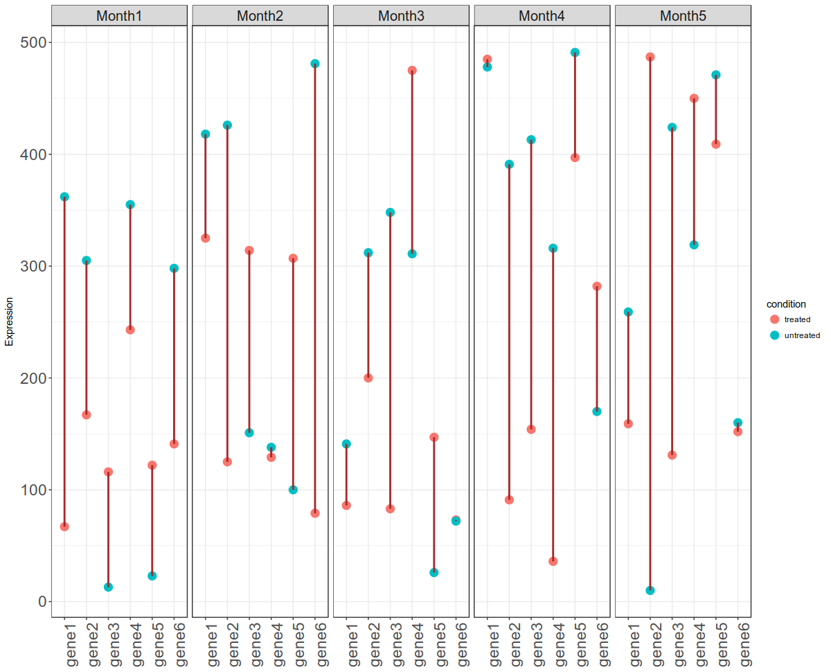
#Now plot genes vertically
library(ggplot2)
ggplot(gx6, aes( id, Expression, color = condition)) +
geom_point(size = 4) +
geom_line(aes(group = id), color = "brown", size = 1) +
facet_wrap(~ time, nrow = 1, ncol = 5) +
theme_bw() +
theme(
axis.text.x = element_text(angle = 90, size = 17),
axis.text.y = element_text(size = 17),
axis.title.x = element_blank(),
strip.text.x = element_text(size = 15)
)

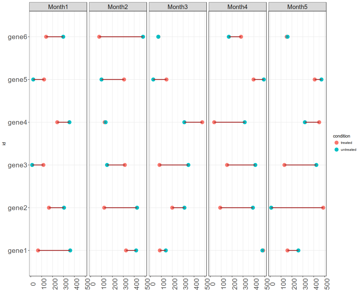
#Now plot genes horizontally
ggplot(gx6, aes(Expression, id, color = condition)) +
          geom_point(size = 4) +
          geom_line(aes(group = id), color = "brown", size = 1) +
          facet_wrap(~ time, nrow = 1, ncol = 5) +
          theme_bw() +
          theme(
             axis.text.x = element_text(angle = 90, size = 17),
             axis.text.y = element_text(size = 17),
             axis.title.x = element_blank(),
             strip.text.x = element_text(size = 15)
            )