There are several methods of representing data esp biological data to end users. Some of them are complex and some, simple. I am not a fan of complex data representations as the underlying data needs comprehension of complex data or incorrect representation of simple data. However, once in a while, such complex figures may be necessary to understand the data. Following one and this image represents the variants per chromosome (SNV, MNV and DIVs). I would like user to go through this topic in the blog to parse VCF into tab file and subsequent data manipulations. I have used clinvar VCF for data and used bcftools to convert VCF to tab file. For graphics, I have used ggplot2.
Object of this tutorial to is represent variants present in clinvar VCF. Please note that the latest clinvar VCF can be downloaded from here for GRCh 38. Variants are categorized under SNV, MNV (Structural variants in general) and DIV (indels) categories and are represented by VC (variant category) VCF. Please follow the instructions on this blog note, to load vcf data into R.
I present two images here: 1) Variants presents in all the chromosomes
2) Variants present per chromosome
First let us list all the variants in clinvar (data frame) using:
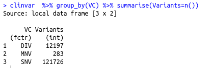
1) Summarize all the variants across all chromosomes:
$ clinvar %>% group_by(VC) %>% summarise(Variants=n())
(Note: use dplyr package for this).
Result would be:

Please note that MNVs are much small in number in compared to both DIV (indels) and SNVs.
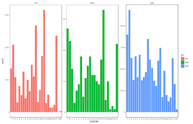 To visualize the same in R using ggplot2, run commands given below:
$ qplot(CHROM, data=clinvar, fill=VC) +
theme(
panel.background=element_rect(colour = "black", fill=NA),
strip.background=element_blank(),
panel.grid.major = element_blank()) +
facet_wrap(~VC,scales = "free")
Now, let us draw all the chromosomes individually and corresponding variants as shown below:
1) Let us draw all variants (SNVs, MNVs and DIVs). Please note that you won't be seeing MNVs as they are very very less in number compared to DIVs and SNVs per chromosome.

Code for getting above image is:
$ ggplot(clinvar, aes(CHROM, fill=VC))+
geom_bar(position = "dodge")+
facet_wrap(~CHROM,ncol=5,nrow = 5, scales = "free")+
theme(
strip.background=element_blank(),
panel.background = element_rect(colour = "black", fill=NA),
axis.text.x =element_blank(),
axis.ticks.x =element_blank(),
panel.grid.major = element_blank())+
labs(title = "Variants in Clinvar", x="Chromosome", y="Number of variants per chromosome")
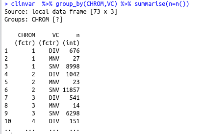
Listing all the variants per chromosome is:
$ clinvar %>% group_by(CHROM,VC) %>% summarise(Variants=n())
Example output is:

Object of this tutorial to is represent variants present in clinvar VCF. Please note that the latest clinvar VCF can be downloaded from here for GRCh 38. Variants are categorized under SNV, MNV (Structural variants in general) and DIV (indels) categories and are represented by VC (variant category) VCF. Please follow the instructions on this blog note, to load vcf data into R.
I present two images here: 1) Variants presents in all the chromosomes
2) Variants present per chromosome
First let us list all the variants in clinvar (data frame) using:
1) Summarize all the variants across all chromosomes:
$ clinvar %>% group_by(VC) %>% summarise(Variants=n())
(Note: use dplyr package for this).
Result would be:

Please note that MNVs are much small in number in compared to both DIV (indels) and SNVs.

$ qplot(CHROM, data=clinvar, fill=VC) +
theme(
panel.background=element_rect(colour = "black", fill=NA),
strip.background=element_blank(),
panel.grid.major = element_blank()) +
facet_wrap(~VC,scales = "free")
Now, let us draw all the chromosomes individually and corresponding variants as shown below:
1) Let us draw all variants (SNVs, MNVs and DIVs). Please note that you won't be seeing MNVs as they are very very less in number compared to DIVs and SNVs per chromosome.
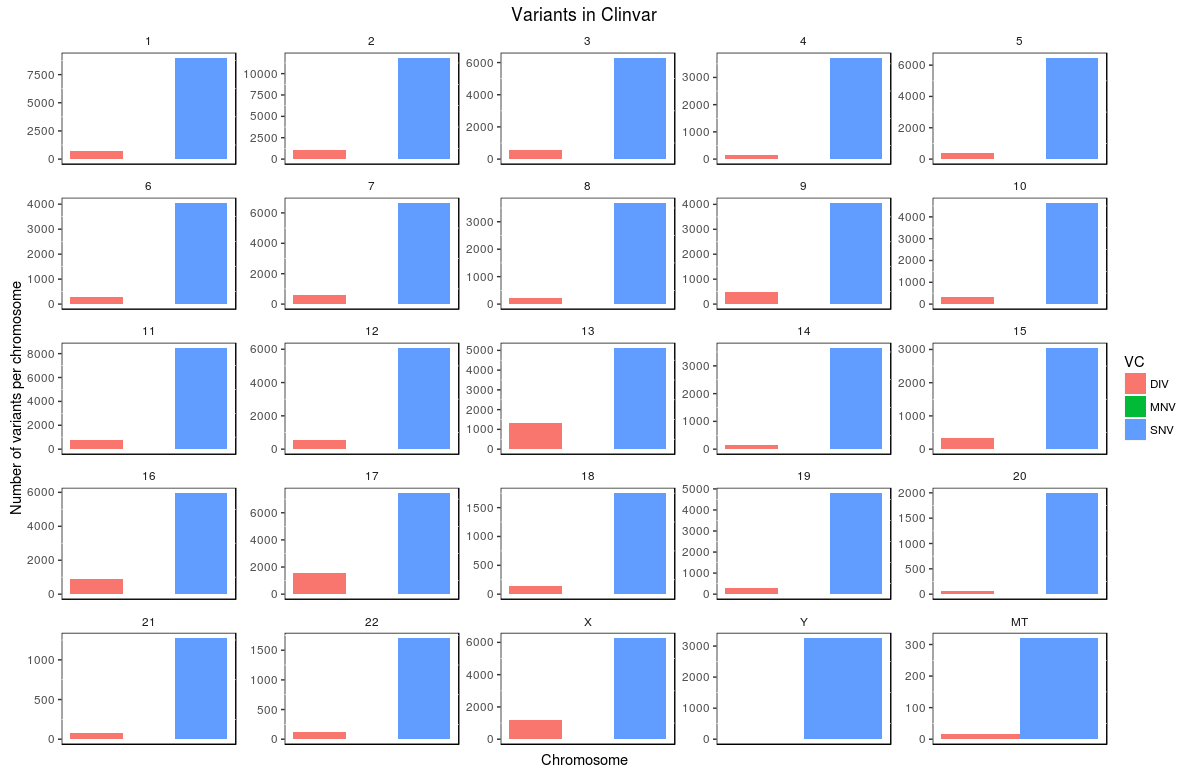
Code for getting above image is:
$ ggplot(clinvar, aes(CHROM, fill=VC))+
geom_bar(position = "dodge")+
facet_wrap(~CHROM,ncol=5,nrow = 5, scales = "free")+
theme(
strip.background=element_blank(),
panel.background = element_rect(colour = "black", fill=NA),
axis.text.x =element_blank(),
axis.ticks.x =element_blank(),
panel.grid.major = element_blank())+
labs(title = "Variants in Clinvar", x="Chromosome", y="Number of variants per chromosome")
Listing all the variants per chromosome is:
$ clinvar %>% group_by(CHROM,VC) %>% summarise(Variants=n())
Example output is: