Recently I came across a request, where researcher requested for plotting data with following description: Multiple genes, each gene with 3 genotypes, each genotype has 3 replicates, each replicate measurement is done at multiple times points. Now the researcher wants to plot for each time point, for each genotype for a single gene. You can download the data from here. Data is copy/pasted at the end of the post. User wants bar and line plot. Bar plot first, line plot later. In either case, user wants mean +/SD plotted over the data.
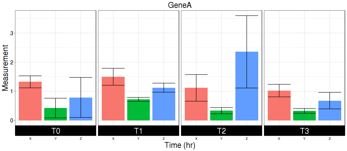
In example data, there are two genes (A,B genes). Each gene has three genotypes (X, Y, Z genotypes), 3 replicates for each genotype (R1, R2, R3) and 4 time points (T0, T1, T2,T3). Now user wants plot each genotype (X, Y, Z) averaging replicates (R1, R2, R3) for each time point (T0, T1, T2, T3). Then plot error bars on for each genotype. What code does is to calculate mean (average), SD and CI for each genotype for each time point. Plot measurement (average) for each genotype and for each time point.
Following is the image:
Code:
=================================
df=read.csv("df1.txt", sep="\t",stringsAsFactors = F)
library(tidyr)
df1=gather(df,"TP","Values",-Gene)
library(stringr)
df2=cbind(df1,str_split_fixed(df1$TP,"_",3))
colnames(df2)[4:6]=c("genotype","time","replicate")
df3=df2[df2$Gene=="A",]
library(Rmisc)
sum_stats <- summarySE(df3, measurevar="Values", groupvars=c("genotype","time"))
colnames(sum_stats)
library(ggplot2)
ggplot(sum_stats, aes(genotype, Values, fill = genotype)) +
geom_bar(stat = "identity") +
facet_wrap(~ time,
ncol = 4,
nrow = 1,
strip.position = "bottom") +
labs(title = "GeneA", x = "Time (hr)", y = "Measurement") +
theme_linedraw() +
theme(
plot.title = element_text(hjust = 0.5, size = 20),
strip.text = element_text(size = 20),
axis.title.y = element_text(size = 20),
axis.title.x = element_text(size = 20),
legend.position = "none",
# axis.text.x = element_blank(),
axis.ticks.x = element_blank(),
axis.text.y = element_text(size = 14)) +
geom_errorbar(aes(ymax = Values + sd, ymin = Values - sd))
==========================
Line graph with Mean +/ SD as shade:

df=read.csv("df1.txt", sep="\t",stringsAsFactors = F)
library(tidyr)
df1=gather(df,"TP","Values",-Gene)
library(stringr)
df2=cbind(df1,str_split_fixed(df1$TP,"_",3))
colnames(df2)[4:6]=c("genotype","time","replicate")
library(Rmisc)
df4=summarySE(df2, measurevar="Values", groupvars=c("time","Gene","genotype"))
library(ggplot2)
ggplot(df4, aes(time, Values, group = genotype, color = genotype)) +
geom_line() +
geom_point() +
facet_wrap( ~ Gene) +
labs(title = "Gene expression over 16 hr", x = "Time (hr)", y = "Measurement") +
theme_linedraw() +
theme(
plot.title = element_text(hjust = 0.5, size = 20),
strip.text = element_text(size = 20),
axis.title.y = element_text(size = 20),
axis.title.x = element_text(size = 20),
axis.text.x = element_text(size = 14),
axis.text.y = element_text(size = 14)
) +
geom_ribbon(aes(ymax = Values + sd, ymin = Values - sd),
alpha = 0.5,
fill = "grey70",
colour=NA
)
Note: Let us say you don't want that hazy thing in scatter plots:
Replace:
geom_ribbon(aes(ymax = Values + sd, ymin = Values - sd),
alpha = 0.5,
fill = "grey70",
colour=NA
)
with :
geom_pointrange(aes(ymax=Values+sd, ymin=Values-sd))"
data:
==================================
Gene X_T0_R1 X_T0_R2 X_T0_R3 X_T1_R1 X_T1_R2 X_T1_R3 X_T2_R1 X_T2_R2 X_T2_R3 X_T3_R1 X_T3_R2 X_T3_R3 Y_T0_R1 Y_T0_R2 Y_T0_R3 Y_T1_R1 Y_T1_R2 Y_T1_R3 Y_T2_R1 Y_T2_R2 Y_T2_R3 Y_T3_R1 Y_T3_R2 Y_T3_R3 Z_T0_R1 Z_T0_R2 Z_T0_R3 Z_T1_R1 Z_T1_R2 Z_T1_R3 Z_T2_R1 Z_T2_R2 Z_T2_R3 Z_T3_R1 Z_T3_R2 Z_T3_R3
A 1.46559502 1.087642983 1.424945196 1.289943948 1.376535013 1.833390311 1.450753714 1.3094609 0.5953716 0.7906009 1.215333041 1.069312467 0.053317766 0.506623748 0.713670106 0.740998252 0.648231834 0.780499252 0.35344654 0.220223951 0.432856978 0.234963735 0.353770497 0.396091395 0.398000559 0.384759325 1.582230097 1.136843842 1.275683837 0.963349308 3.765036263 1.901023385 1.407713024 0.988333629 0.618606729 0.429823986
B 0.220140568 0.237500819 0.21066267 0.207778662 0.488774258 0.182798731 0.247576125 0.390028842 1.007079177 0.730242116 1.012914813 0.780421013 3.316414959 3.599442788 2.516735845 1.444496448 0.097957459 0.187840968 1.190274584 1.367784148 1.403057729 1.232129062 0.885122768 1.333921747 1.286528398 1.122251177 0.697419716 0.804552001 1.227821594 0.968589683 0.477443352 0.832736132 0.911920317 1.095130142 0.497458337 0.471389536=======================================================