Circos plots are high density, circular plots visualizing data at a higher level. Tiling, expression, variations (sequence, structure and CN) data can be drawn using Circos maps. However, circular representation of genome is not new. For eg. Bacterial genomes, Plasmids were represented by circular diagrams earlier. But they are not as dense as circos handles. One can know more about circos at http://circos.ca/.
In R, circos plots can be drawn using either RCircos and OmicCircos. Incidentally, both are from same institute. I used both of them. Here RCircos is explained.
For drawing circos plots in R, following packages and data is necessary:
1) RCircos (http://cran.r-project.org/web/packages/RCircos/index.html).
2) Ideogram data for the organism of interest. Example given below is for mouse (Mus musculus)
3) Gene symbols with coordinates for entire genome or genes that are affected in user study (for differential genes, genes with clinical SNPs)
4) User data. In this example, mouse expression data is used and download it here: https://drive.google.com/file/d/0B0MpwluEDxNuMEZ4MU9aUkNyMTg/edit?usp=sharing.
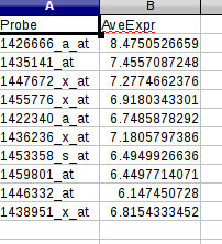
Data contains two columns: Affymetrix probes and their differential expression values (after analysis, between two groups) We will be using only probes and their expression values in drawing circos map.
In general circos map will have following components:
1) Ideogram map
2) Gene symbols
3) Connectors between ideogram map and gene symbols (i.e arrows from ideogram map to gene symbols)
4) User tracks
 In general (for RCircos), ideogram map is track zero. It has two sides: in and out. From ideogram map, towards inside, tracks would start with 1 and as you go to the center, track numbers increase. From ideogram map, towards outside, tracks would start 1 and as you go away from ideogram map, track numbers increase.

First user needs to draw ideogram and ideogram data (for several organisms) can be obtained from UCSC genome browser tables. Here I have used data for mouse (Mus musculus). Format expected is: Chromomosome, chromStart, chromEnd, name, gieStain and file I used can be downloaded from here: https://drive.google.com/file/d/0B0MpwluEDxNudEZuUlRCQmlSZGs/edit?usp=sharing.
Before drawing Circos map, following things needs to be done:
1) For the affymetrix probes, we need to get their coordinates, gene name, chromosome number. For this we would be use biomart service
2) Merge annotation file (from biomart) with expression values.
Let us fetch the annotations for differentially expressed mouse probes and the link to download probes is (given above): https://drive.google.com/file/d/0B0MpwluEDxNuMEZ4MU9aUkNyMTg/edit?usp=sharing. Shared file is tar.gz and it contains top 10 significant, differentially expressed probes and their expression values.

Steps to load probes and their expression values:
1) Download the data, unzip and untar to get a text file with name:
2) Import the data in R
$ top=read.table("toptable.txt", header=TRUE)
Steps to fetch probe set information using biomart in R:
1) Load biomart package in R
$ library(biomaRt)
2) Use ensembl mart
$ ensembl=useMart("ensembl")
3) Use mouse gene database in ensembl mart
$ mm_ensembl=useDataset("mmusculus_gene_ensembl", mart=ensembl)
4) Define what we need from ensembl mouse database and store them in an object
$ mm_attr1=listAttributes(mm_ensembl)[c(98,6:8,60),]
We need following information: Original probes that are used for querying database, Chromosome name, Gene start, Gene end and Gene symbol (MGI). Numbers 98, 6, 7, 8 and 60 code for these in the database.
5) Fetch the information for the probes, once we define what we want and store the information
$ bm_mm_ensembl=getBM(attributes=c(mm_attr1[,1]),filters='affy_mouse430_2',values=top[1], mart=mm_ensembl)

6) Change the first column heading (this would be helpful when merging two files later: user uploaded file and annotations from Ensembl)
$ colnames(bm_mm_ensembl)[1]="Probe"
7) Extract chromosome numbers, start position, end position and gene symbol and sort chromosome number and start position. Store the information. This would be used in circos plot in drawing genes track.
$ gene_label=bm_mm_ensembl[order(bm_mm_ensembl$chromosome_name,bm_mm_ensembl$start_position),][2:5]
8) Change the column names for better representation.
$ colnames(gene_label)=c("Chromosome","Start", "End", "Symbol")

9) Merge probe expression data with annotation data i.e to get chromosome number, coordinates, symbol and expression values for each probe. Two data frames , top (imported data) and bm_mm_ensembl (annotation data) are merged by common column (common column heading- "Probe").
$ final_expr=merge(top,bm_mm_ensembl, by="Probe")[,c(3:6,2)]
10) Being careful, sort the values by chromosome and start coordinates
$ final_expr1=final_expr[order(final_expr$chromosome_name,final_expr$start_position),]
11) Change the column names for better representation
$ colnames(final_expr1)=c("Chromosome", "Sart", "End", "Symbol","FoldChange")
Please note that names should not have any spaces.
Now let us draw the R Circos map for the probes and their expression values:
12) Import ideogram values in to R and store them.
$ mi=read.delim2("mouse_ideogram_ucsc.txt", head=TRUE)
13) Load RCircos package in R and rcircos package can be down loaded from http://cran.r-project.org/web/packages/RCircos/index.html. Package is available in Bioc repositories.
$ library(RCircos)
14) Define core components in drawing: number of tracks, chromosomes to be excluded in drawing (if there are any), how may tracks we need inside and how many outside and ideogram information.
$ RCircos.Set.Core.Components(cyto.info=mi, chr.exclude=NULL, tracks.inside=10, tracks.outside=2)
15) Since we want the map be drawn and stored as an image file, provide a name for the file, it's resolution.
$ png(file="mm_expression_demo.png", height=8, width=8, unit="in",type="cairo", res=300)
Please note that this start drawing image in the back ground (in R parlance, this would open a device) and all the subsequent drawings/steps would be performed in the background and user would not be able to see those in terminal. User has to stop drawing images (i. e close the device) at the end to see final image.
16) Start drawing the map
$ RCircos.Set.Plot.Area();
17) Supply the title to the image
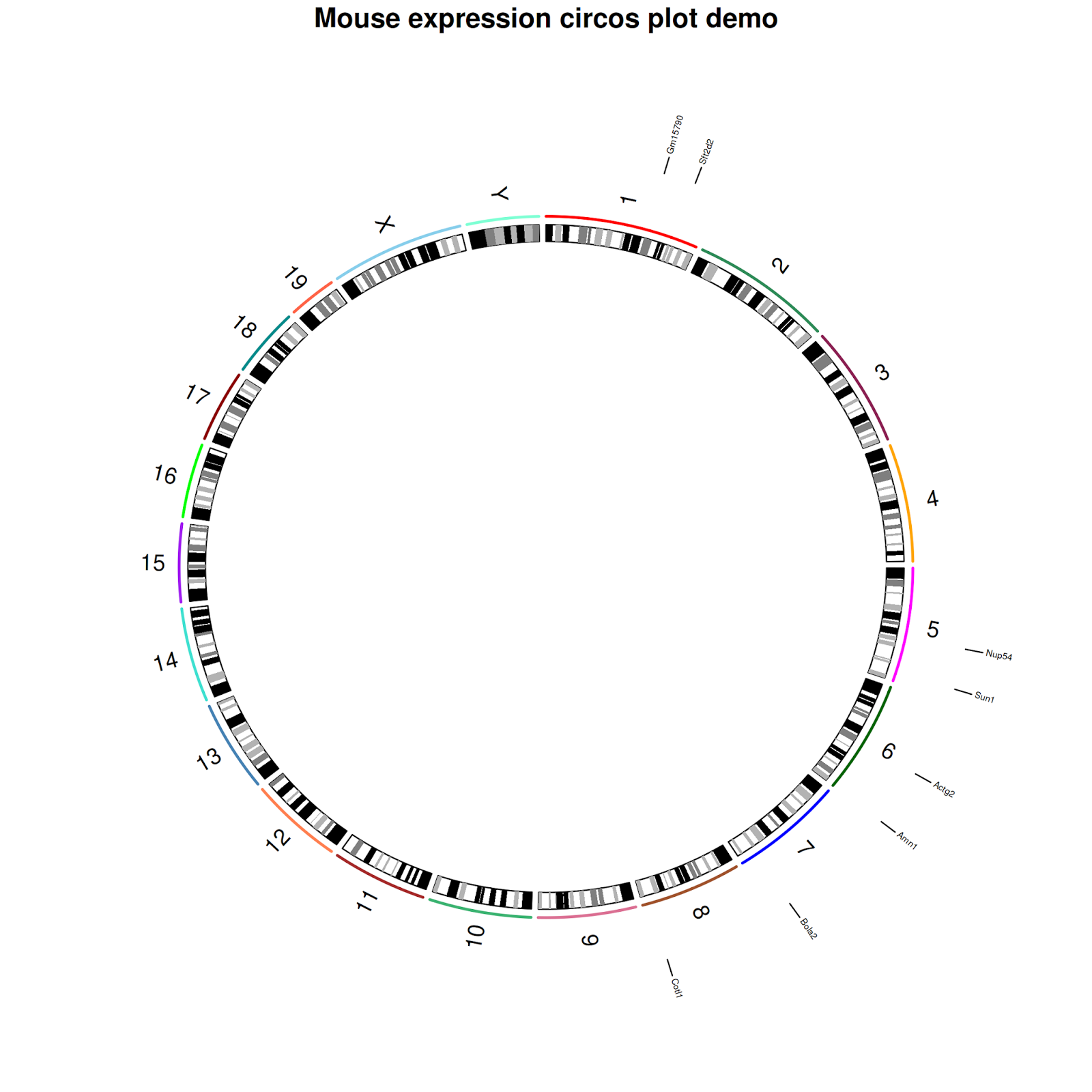
$ title("Mouse expression circos plot demo");
18) Draw the ideogram
$ RCircos.Chromosome.Ideogram.Plot();

19) Display gene names on the ideogram plot, out side
$ RCircos.Gene.Name.Plot(gene.data=gene_label,name.col=4,track.num=2, side="out")
Please note that user can draw either all the genes (in mouse genome) or selected set of genes (of user choice). Format to be followed is: 4 columns with Chromomsome, Start, End,Symbol
20) Connect the gene names with ideogram plots by connectors, on out side
$ RCircos.Gene.Connector.Plot(genomic.data=gene_label,track.num=1, side="out")
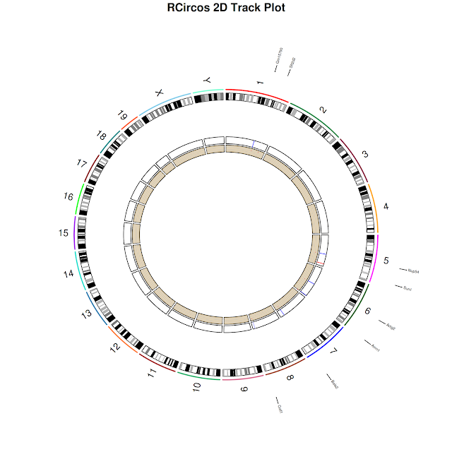
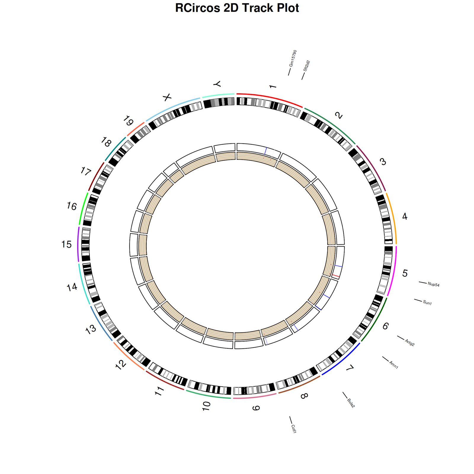
 21) Plot probe data as heatmap (in track 5).
$ RCircos.Heatmap.Plot(heatmap.data=final_expr1, data.col=5,track.num=5, side="in")
22) Plot probe data as scatter plot (in track 6)
RCircos.Scatter.Plot(scatter.data=final_expr1, data.col=5,track.num=6, side="in", by.fold=1)
 23) Stop drawing image in the back ground (i.e close the device).
$ dev.off()
Please note that RCircos is strict about data type (for eg. chromosome coordinates, expression values should be numeric, integers, but not factors.) and sorting (for chromosome sorting)
In R, circos plots can be drawn using either RCircos and OmicCircos. Incidentally, both are from same institute. I used both of them. Here RCircos is explained.
For drawing circos plots in R, following packages and data is necessary:
1) RCircos (http://cran.r-project.org/web/packages/RCircos/index.html).
2) Ideogram data for the organism of interest. Example given below is for mouse (Mus musculus)
3) Gene symbols with coordinates for entire genome or genes that are affected in user study (for differential genes, genes with clinical SNPs)
4) User data. In this example, mouse expression data is used and download it here: https://drive.google.com/file/d/0B0MpwluEDxNuMEZ4MU9aUkNyMTg/edit?usp=sharing.
Data contains two columns: Affymetrix probes and their differential expression values (after analysis, between two groups) We will be using only probes and their expression values in drawing circos map.
In general circos map will have following components:
1) Ideogram map
2) Gene symbols
3) Connectors between ideogram map and gene symbols (i.e arrows from ideogram map to gene symbols)
4) User tracks


First user needs to draw ideogram and ideogram data (for several organisms) can be obtained from UCSC genome browser tables. Here I have used data for mouse (Mus musculus). Format expected is: Chromomosome, chromStart, chromEnd, name, gieStain and file I used can be downloaded from here: https://drive.google.com/file/d/0B0MpwluEDxNudEZuUlRCQmlSZGs/edit?usp=sharing.
Before drawing Circos map, following things needs to be done:
1) For the affymetrix probes, we need to get their coordinates, gene name, chromosome number. For this we would be use biomart service
2) Merge annotation file (from biomart) with expression values.
Let us fetch the annotations for differentially expressed mouse probes and the link to download probes is (given above): https://drive.google.com/file/d/0B0MpwluEDxNuMEZ4MU9aUkNyMTg/edit?usp=sharing. Shared file is tar.gz and it contains top 10 significant, differentially expressed probes and their expression values.
Steps to load probes and their expression values:
1) Download the data, unzip and untar to get a text file with name:
2) Import the data in R
$ top=read.table("toptable.txt", header=TRUE)
Steps to fetch probe set information using biomart in R:
1) Load biomart package in R
$ library(biomaRt)
2) Use ensembl mart
$ ensembl=useMart("ensembl")
3) Use mouse gene database in ensembl mart
$ mm_ensembl=useDataset("mmusculus_gene_ensembl", mart=ensembl)
4) Define what we need from ensembl mouse database and store them in an object
$ mm_attr1=listAttributes(mm_ensembl)[c(98,6:8,60),]
We need following information: Original probes that are used for querying database, Chromosome name, Gene start, Gene end and Gene symbol (MGI). Numbers 98, 6, 7, 8 and 60 code for these in the database.
5) Fetch the information for the probes, once we define what we want and store the information
$ bm_mm_ensembl=getBM(attributes=c(mm_attr1[,1]),filters='affy_mouse430_2',values=top[1], mart=mm_ensembl)

6) Change the first column heading (this would be helpful when merging two files later: user uploaded file and annotations from Ensembl)
$ colnames(bm_mm_ensembl)[1]="Probe"
7) Extract chromosome numbers, start position, end position and gene symbol and sort chromosome number and start position. Store the information. This would be used in circos plot in drawing genes track.
$ gene_label=bm_mm_ensembl[order(bm_mm_ensembl$chromosome_name,bm_mm_ensembl$start_position),][2:5]
8) Change the column names for better representation.
$ colnames(gene_label)=c("Chromosome","Start", "End", "Symbol")

9) Merge probe expression data with annotation data i.e to get chromosome number, coordinates, symbol and expression values for each probe. Two data frames , top (imported data) and bm_mm_ensembl (annotation data) are merged by common column (common column heading- "Probe").
$ final_expr=merge(top,bm_mm_ensembl, by="Probe")[,c(3:6,2)]
10) Being careful, sort the values by chromosome and start coordinates
$ final_expr1=final_expr[order(final_expr$chromosome_name,final_expr$start_position),]
11) Change the column names for better representation
$ colnames(final_expr1)=c("Chromosome", "Sart", "End", "Symbol","FoldChange")
Please note that names should not have any spaces.
Now let us draw the R Circos map for the probes and their expression values:
12) Import ideogram values in to R and store them.
$ mi=read.delim2("mouse_ideogram_ucsc.txt", head=TRUE)
13) Load RCircos package in R and rcircos package can be down loaded from http://cran.r-project.org/web/packages/RCircos/index.html. Package is available in Bioc repositories.
$ library(RCircos)
14) Define core components in drawing: number of tracks, chromosomes to be excluded in drawing (if there are any), how may tracks we need inside and how many outside and ideogram information.
$ RCircos.Set.Core.Components(cyto.info=mi, chr.exclude=NULL, tracks.inside=10, tracks.outside=2)
15) Since we want the map be drawn and stored as an image file, provide a name for the file, it's resolution.
$ png(file="mm_expression_demo.png", height=8, width=8, unit="in",type="cairo", res=300)
Please note that this start drawing image in the back ground (in R parlance, this would open a device) and all the subsequent drawings/steps would be performed in the background and user would not be able to see those in terminal. User has to stop drawing images (i. e close the device) at the end to see final image.
16) Start drawing the map
$ RCircos.Set.Plot.Area();
17) Supply the title to the image
$ title("Mouse expression circos plot demo");
18) Draw the ideogram
$ RCircos.Chromosome.Ideogram.Plot();

19) Display gene names on the ideogram plot, out side
$ RCircos.Gene.Name.Plot(gene.data=gene_label,name.col=4,track.num=2, side="out")
Please note that user can draw either all the genes (in mouse genome) or selected set of genes (of user choice). Format to be followed is: 4 columns with Chromomsome, Start, End,Symbol
20) Connect the gene names with ideogram plots by connectors, on out side
$ RCircos.Gene.Connector.Plot(genomic.data=gene_label,track.num=1, side="out")
$ RCircos.Heatmap.Plot(heatmap.data=final_expr1, data.col=5,track.num=5, side="in")
22) Plot probe data as scatter plot (in track 6)
RCircos.Scatter.Plot(scatter.data=final_expr1, data.col=5,track.num=6, side="in", by.fold=1)
$ dev.off()
Please note that RCircos is strict about data type (for eg. chromosome coordinates, expression values should be numeric, integers, but not factors.) and sorting (for chromosome sorting)