This is not a bioinformatics note, rather a generic note. Some times we may have to parse data from files from binary formats such as .doc, .docx, .xls, .xls, .pdf etc. In this note, let us analyze the data from a pdf. Source of PDF is results announced by Andhra Pradesh Government (India) for examination conducted for Assistant professor posts in government universities in lifesciences. (Link for PDF: https://www.psc.ap.gov.in/(S(cy3miignuzcio4zg5za5wyd4))/Documents/AsstProf/Marks/LIFE%20SCIENCESwebformat.pdf)
Note: This note is not meant to draw any conclusions and all conclusions based on this data will be erroneous as the data is incomplete. This note is strictly meant for data parsing from a public pdf into R. That is all it is. Do not use the file for any other statistical and/or social conclusions.
PDF page has several information for each candidate: S.No, Hall ticket number, Community information, DOB, Gender, Marks in Paper1 and Paper2, Adjusted questions, Total marks out of 300. We will do following steps in this note:
- Import the data
- Construct a data frame (from matrix)
- Chuck out the unnecessary information
- Calculate each candidate age
- Create age range
- Some basic visualizations using ggplot and basic plotting
Now let us get into the work. Before you get into the work, download the PDF from the link:
=================
# This is because Hall ticket numbers are large numbers and R will convert them to exponential (e) numbers.
> options(scipen = 999)
# Load libraries
> library(tabulizer)
# Use extract tables function from Tabulizer package. This would extract the tables in to list.
> result=extract_tables("LIFE SCIENCESwebformat.pdf")
# This would convert the data into matrix. Let us keep this as matrix for pruning
> result1 <- do.call(rbind, result[-length(result)])
# Remove first two rows. First two rows are not necessary for the analysis
> result1=result1[-c(1:2),]
# From remaining rows, make the first row as header and then delete the first row.
> colnames(result1)=result1[1,]
> result1=result1[-1,]
# Convert the data from matrix to data frame
> result1=as.data.frame(result1)
# Load libraries for data manipulation
> library(tidyr)
> library(dplyr)
> library(lubridate)
# Select DOB, Marks and Gender columns. Convert DOB as date format, calculate the age and create age range for every 5 yr. Since lowest age was 21, for the sake of uniform ranges, 20 (21-1) was taken as lowest age for creating age ranges.
>result2 = result1 %>%select (c(DOB, Gender, `Total Marks 300`)) %>%
mutate_at(vars(`Total Marks 300`), funs(as.numeric(as.character(.))))%>%
mutate_at(vars("DOB"), funs(as.Date(., "%d/%m/%Y"))) %>%
mutate(age = time_length(Sys.Date() - DOB, "years")) %>%
mutate(range = cut(age, breaks = seq(floor(min(age) - 1), ceiling(max(age)), by = 5)))
# Now that we have the dataframe we have, let us run some basic analysis.
# Total number of candidates attended
> result2 %>% summarise(Candidates=n())
Candidates
1 2137
# Total number of males and females attended:
> result2 %>% group_by(Gender) %>% summarise(Candidates=n())
# A tibble: 3 x 2
Gender Candidates
<fct> <int>
1 F 946
2 M 1190
3 T 1
It seems there is one third gender person attended.Now let us look at the average (mean) age of the each gender category.
> result2 %>% group_by(Gender)%>% summarise(Candidates= n(), "Average age (in yrs)"=mean(age))
# A tibble: 3 x 3
Gender Candidates `Average age (in yrs)`
<fct> <int> <dbl>
1 F 946 35.9
2 M 1190 35.8
3 T 1 32.1
# A tibble: 3 x 3
Gender Candidates `Average age (in yrs)`
<fct> <int> <dbl>
1 F 946 35.9
2 M 1190 35.8
3 T 1 32.1
It seems average age of female is 35.9 and male is 35.8. Not much difference. Now let us break down age into age range wise attendance.
> result2 %>% group_by(range)%>% summarise(Candidates= n()) %>% spread(range, Candidates)
# A tibble: 1 x 8
`(20,25]` `(25,30]` `(30,35]` `(35,40]` `(40,45]` `(45,50]` `(50,55]` `(55,60]`
<int> <int> <int> <int> <int> <int> <int> <int>
36 256 692 694 313 103 34 9
# Interesting. We have attendance from 20-25 to 55-60. Now let us break this down by gender.
> result2 %>%
+ group_by(range, Gender)%>%
+ summarise(Candidates= n()) %>%
+ spread(range, Candidates)
# A tibble: 3 x 9
Gender `(20,25]` `(25,30]` `(30,35]` `(35,40]` `(40,45]` `(45,50]` `(50,55]` `(55,60]`
<fct> <int> <int> <int> <int> <int> <int> <int> <int>
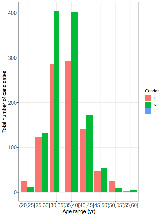
1 F 25 124 287 292 141 48 25 4
2 M 11 132 404 402 172 55 9 5
3 T NA NA 1 NA NA NA NA NA
# This is very interesting because we have third gender person in age group of 30-35. Let us look at the histogram.
>result2 %>%
group_by(range)%>%
summarise(Candidates= n()) %>%
ggplot(aes(range,Candidates, fill=range))+
geom_bar(stat="identity")+
theme_bw()+
theme(axis.text.x = element_text(size=14),
axis.text.y = element_text(size=14),
axis.title.x = element_text(size=14),
axis.title.y = element_text(size=14))+
labs(x = "Age range (yr)", y= "Total number of candidates")
Now that we have seen people between 30-40 age attended more, let us break it further into gender wise applications.
> result2 %>%
group_by(range, Gender)%>%
summarise(Candidates= n()) %>%
ggplot(aes(range,Candidates, fill=Gender))+
geom_histogram(stat="identity", position = "dodge")+
theme_bw()+
theme(axis.text.x = element_text(size=14),
axis.text.y = element_text(size=14),
axis.title.x = element_text(size=14),
axis.title.y = element_text(size=14))+
labs(x = "Age range (yr)", y= "Total number of candidates")
Now we have seen the age distribution, it seems 30-40 age group people applied for the job. Now it seems there are certain people who are absent. In the marks columns, they are marked "Absent". Let us count how many of the total applied people appeared for the exam.
> table(result1$`Total Marks 300`=='Absent')
FALSE TRUE
1574 563
FALSE TRUE
1574 563
563 people didn't attend the exam. Let us count the males and females who appeared for the exam. For this we will remove absent people and then count females and males. Before that let us create an object removing absent candidates. Since we converted marks columns to numbers, absent are converted to na. Let us remove them and store it in a different object.
> result3=result2 %>% na.omit()
> result3 %>%select(-c(DOB)) %>% group_by(Gender) %>% summarise(n=n())
# A tibble: 3 x 2
Gender Total
<fct> <int>
1 F 701
2 M 872
3 T 1
# A tibble: 3 x 2
Gender Total
<fct> <int>
1 F 701
2 M 872
3 T 1
Interesting to see that males appeared for exam more in number compared to females, in attending the exam and matches with the application trend. Let us calculate average age and average marks for each gender.
>result3%>%select(-c(DOB))%>%group_by(Gender)%>% summarise_at (c ("Total Marks 300", "age"), mean, na.rm=T)
# A tibble: 3 x 3
Gender `Total Marks 300` age
<fct> <dbl> <dbl>
1 F 78.3 36.2
2 M 83.7 35.9
3 T 72.8 32.1
# A tibble: 3 x 3
Gender `Total Marks 300` age
<fct> <dbl> <dbl>
1 F 78.3 36.2
2 M 83.7 35.9
3 T 72.8 32.1
Now let us do boxplot of data. Let us plot all the marks, but gender wise.
> ggplot(result3, aes(x =Gender, y = `Total Marks 300`, fill=Gender))+
geom_boxplot()+
scale_x_discrete(labels=c("F"="Female","M"="Male","T"="Trans"))+
theme_bw()+
geom_boxplot()+
scale_x_discrete(labels=c("F"="Female","M"="Male","T"="Trans"))+
theme_bw()+
theme(axis.text.x = element_text(size=14),
axis.text.y = element_text(size=14),
axis.title.x = element_text(size=14),
axis.title.y = element_text(size=14))+
labs(x = "Age range (yr)", y= "Total number of candidates")
axis.text.y = element_text(size=14),
axis.title.x = element_text(size=14),
axis.title.y = element_text(size=14))+
labs(x = "Age range (yr)", y= "Total number of candidates")
