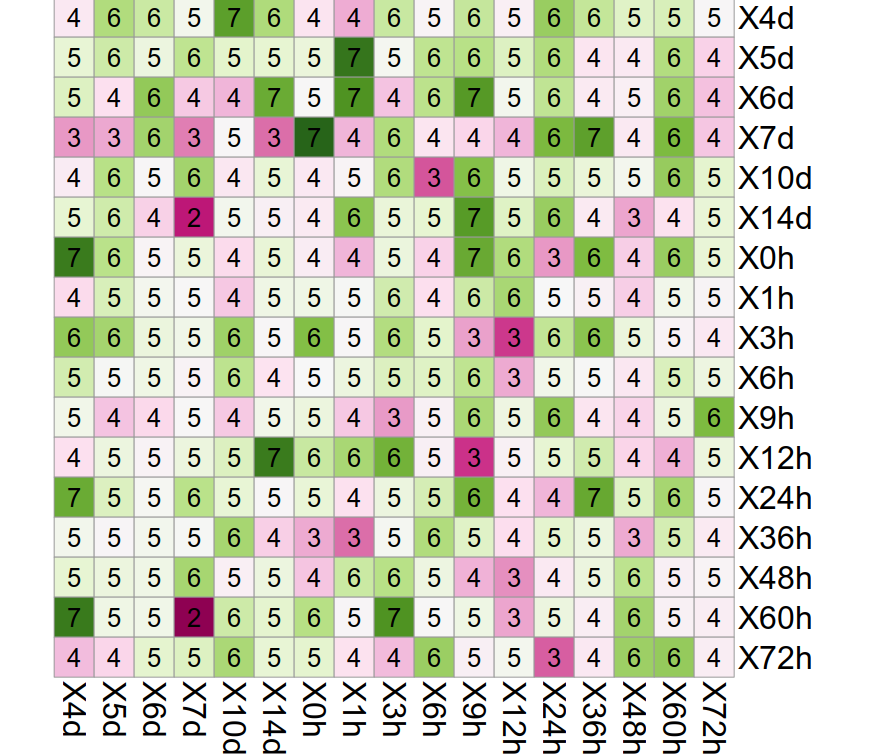
Some times, you need to plot expression numbers, not the trends, across samples. Now let us simulate a data frame and then plot it in R. Let me first show the output to be clear about output.
===========================
$ library(pheatmap)
$ library(RColorBrewer)
$ samples=c(paste0("X",c(4:7,10,14),"d"), paste0 ("X",c(0,1,3,6,9,12,24,36,48,60,72),"h"))
$ df3=data.frame(replicate (17,rnorm(17,5,1)), row.names = samples)
$ colnames(df3)=samples
$ pheatmap(
df3,
display_numbers = T,
cellwidth = 30,
cellheight = 30,
cluster_row = F,
cluster_col = F,
show_rownames = T,
show_colnames = T,
fontsize = 24,
number_color = "black",
color = colorRampPalette(brewer.pal(11, "PiYG"))(289),
number_format="%.f",
legend = F
)
====================================
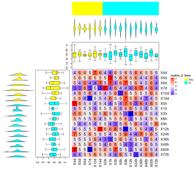
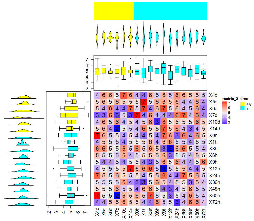
Output is as shown in 2nd image. Now let us generate complex image as shown in first image. For this we would be using complexheatmap package in R.
=====================================
# Create the data frame as above. Do not load pheatmap library.
> suppressPackageStartupMessages(library(ComplexHeatmap))
> suppressPackageStartupMessages(library(circlize))
## Create row annotations
> df3rowann <-
HeatmapAnnotation(
violin = anno_density(
data.matrix(df3),
type = "line",
gp = gpar(fill = rep(col_col$time, c(6, 11))),
which = "row"
),
boxplot = anno_boxplot(
data.matrix(df3),
border = TRUE,
gp = gpar(fill = rep(col_col$time, c(6, 11))),
pch = ".",
axis = TRUE,
axis_side = "bottom",
axis_gp = gpar(fontsize = 12),
which = "row"
),
which = "row",
width = unit(8, "cm")
)
## Create column annotations.
df3topCol <-
HeatmapAnnotation(
violin = anno_density(
data.matrix(df3),
type = "violin",
gp = gpar(fill = rep(col_col$time,c(6,11)))),
boxplot = anno_boxplot(
data.matrix(df3),
border = TRUE,
gp = gpar(fill = rep(col_col$time,c(6,11))),
pch = ".",
axis = TRUE,
axis_side = "left",
axis_gp = gpar(fontsize = 12),
),
which = "col",
df = colann, col = col_col,
)
## Main plot
df3rowann + Heatmap(
df3,
cell_fun = function(j,i,x, y, width, height, fill) {
grid.text(sprintf("%.f", df3[i,j]), x, y, gp = gpar(fontsize = 14))
},
cluster_rows = FALSE,
cluster_columns = FALSE,
top_annotation_height = unit(8, "cm"),
top_annotation = df3topCol,
)
======================================
Image is as in first image. The issue with complexheatmap compared to pheatmap is that it is not easy to display numbers in heatmap without some complex code. On the other hand, pheatmap doesn't have column and row annotation capabilites as complexheatmap.
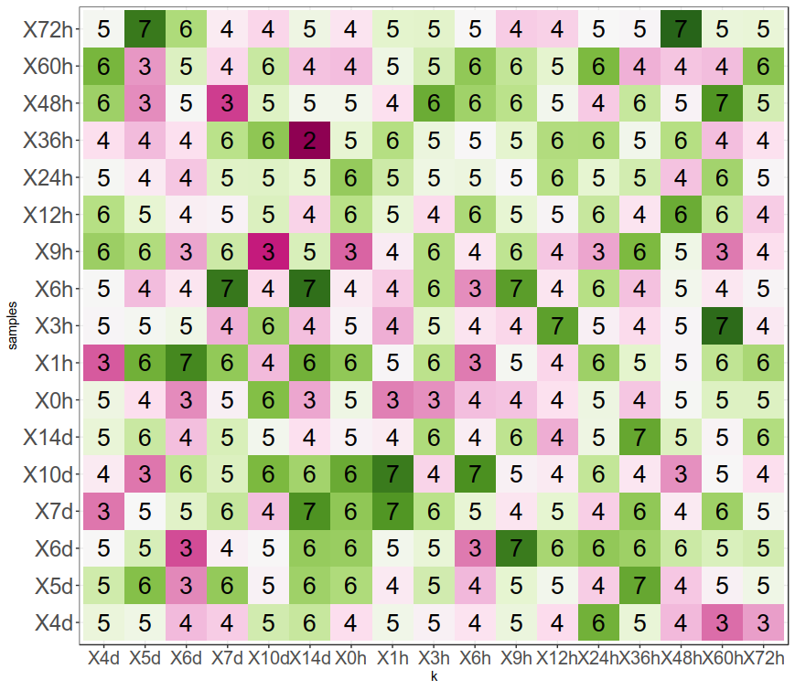
Now the question is can we do it in ggplot. Remember simulation of data involves random number generation. Hence ggplot image numbers and above numbers may not match, but code runs fine.
==========================
$samples=c(paste0("X",c(4:7,10,14),"d"),paste0("X",c(0,1,3,6,9,12,24,36,48,60,72),"h"))
$ df3=data.frame(replicate (17,rnorm(17,5,1)), samples = samples)
$ colnames(df3)[-ncol(df3)]=samples
$ df3$samples=factor(df3$samples, levels=df3$samples)
$ row.names(df3)=samples
$ library(ggplot2)
$ library(tidyr)
$ library(RColorBrewer)
$ df4=gather(df3, k,v, -samples)
$ df4$k=factor(df4$k, levels=unique(df4$k))
$ ggplot(df4, aes (k, samples, label=round(v,0), fill=v)) +
geom_tile()+
geom_text(size=7)+
scale_fill_gradientn (colours = colorRampPalette (brewer.pal (11, "PiYG")) (289), guide="none")+
theme_bw()+
theme(axis.text.x =element_text(size=15),
axis.text.y=element_text(size=18))
==============================================
Let us say we don't want any coloring, we just want to display the numbers and numbers are as per their size and colored from low to high with light color to strong color. Let us do this in ggplot2.

# Generation of data frame is same as above in ggplot2 code. Proceed till df4.
$ ggplot(df4, aes( k, samples, label = round(v,0), colour = v, size = v)) +
geom_text()+
scale_colour_distiller(palette = "Dark2", guide = "none")+
scale_size_identity()+
theme_bw()
====================================