Most of the gene expression studies result in heatmaps for publications, presentations and posters. There are several tools for generating heatmaps. Most of the tools expect a matrix (also called an expression matrix). Matrix will have values (integers) for each gene in rows i.e genes are present in rows and corresponding expression values are presented against them row wise and corresponding sample name would be in columns. In summary, genes in rows, samples in columns and corresponding values against appropriate gene and sample. Think of it as point drawn against x, y coordinates.

Now one of the easiest heatmap generating library in R is pheatmap. However, once we get to heatmpap, we would need more functions and this where complexheatmap shines. For quick heatmap, pheatmap shines and for complex heatmaps, complexheatmap shines. One of the user requirements to change the font color as per cutoff. In this case, user wants to highlight genes (row names) with color (green and red) indicating regulation (up and down). Let us do this.

#Load libraries
library(grid)
library(pheatmap)

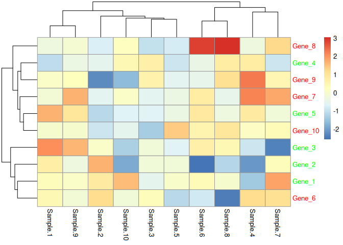
Now let us simulate some expression data with 10 genes, 10 samples and store it as data frame

data <- replicate(10, rnorm(10))
rownames(data) <- paste0("Gene_", c(1:nrow(data)))
colnames(data) <- paste("Sample", c(1:ncol(data)))
data=data.frame(data)

In general, upregulation and downregulation is based on fold change values and they come after the analysis. Since this is a simulated data, let us add a column, with up and down statuses for the sake of simplicity. Now data frame has expression values and regulation status (up or down)

data$status=rep(c("up","down"), each=dim(data)[1]/2)

Now that we have created status, let us give conditional colors. If the regulation is up, it is represented by green color, and red color represents down regulation.

data$colors=ifelse(data$status=="up","green","red")

Remember the data is in first 10 columns (10 samples) only. So let us create heatmap from first 10 columns. Now that we have looked at heatmap, let us store the heatmap as an object

e=pheatmap(data[,1:10])

Now we need to define the colors. Unfortunately, we can’t take the colors as such as there is grouping while drawing heatmap and grouping disturbs order of the data frame. Hence we need to take the genes and their order of appearance from heatmap object, rearrange the data frame as per heatmap and take colors from the rearranged data frame. Final object would be stored in cols, contains colors and exactly in the same order as genes in heatmap object. We need to identify the grob in which row names are located in heatmap object. In this case, it is located in grob 5. One can get it in gtable of the heatmap object.

cols=data[order(match(rownames(data), e$gtable$grobs[[5]]$label)), ]$colors

Now let us assign the colors to graph object

e$gtable$grobs[[5]]$gp=gpar(col=cols)

Now redraw the heatmap

e