As mentioned in earlier notes here, there are scientists who use Tophat-HTseq-DESeq2 pipeline instead of Tophat-Cufflinks-Cummerbund pipeline. I realized that there are a variety of predefined bpipe work flows and are made available for end user here (Program and dependencies installations are around ~400mb in Ubuntu 14.4).
I am posting shell script (bash) coupled with R script for analysis. In this note, you will find pipeline for RNAseq data analysis using Tophat, HTseq and DESeq2 analysis. Please keep following notes in mind:
I am posting shell script (bash) coupled with R script for analysis. In this note, you will find pipeline for RNAseq data analysis using Tophat, HTseq and DESeq2 analysis. Please keep following notes in mind:
1) This notes (and this blog) is meant for biologists, not for programmers or statisticians.
2) This notes is an example, not an optimized pipeline
3) This notes uses data available for public consumption. Hence data derived and demo pipeline used in this note are for public consumption without any prejudice.
Let us jump into the work flow. Work flow is outlined below:

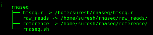
This notes contain a bash script including an R script within it. Please make sure that reference files are in a folder called "reference" and raw reads are in a folder, titled "raw_reads". Execute the shell script in a directory which has reference and raw_reads with in it. Please note that cutadapt QC output is same as that raw reads.
Original files including raw reads (two groups: MeOH and R3H paired end reads, with 3 replicates), reference gtf and reference fasta can be downloaded here.
Download the raw files (12 fastqc files in total) and store them in a folder titled "raw_reads". Download fasta and gtf file and store them in a folder titled "reference". Run the following script. Please keep the r script file, raw_files folder and reference folder, in a single folder and run the script. Please note that I haven't used threads or core options for each program.
=================
bash script starts here
=================
#For loop to declare each sample
for i in $(ls ./raw_reads | grep ^[^d]| rev | cut -c 10- | rev | uniq)
do
# Make direcotry for fastqc
mkdir -p ${i%}fastqc
# Run fastqc
fastqc -o ./${i%}fastqc -f fastq ./raw_reads/${i%}_R1.fastq ./raw_reads/${i%}_R2.fastq
# Make directory to store cutadapt results
mkdir -p cutadapt
#Run cutadapt
cutadapt -a AGATCGGAAGAGCGGTTCAGCAGGAATGCCGAGACCGATC --quality-cutoff=20 --format=fastq -o ./cutadapt/${i%}_R1.cutadapt.fastq -p ./cutadapt/${i%}_R2.cutadapt.fastq ./raw_reads/${i%}_R1.fastq ./raw_reads/${i%}_R2.fastq
# Run top hat and save the out with directory extension _tophatout
tophat2 --no-coverage-search -o ./${i%}_tophatout -G ./reference/genes_chr12.gtf -p 2 ./reference/chr12 ./cutadapt/${i%}_R1.cutadapt.fastq ./cutadapt/${i%}_R2.cutadapt.fastq --rg-id ${i} --rg-sample ${i%} --rg-library rna-seq --rg-platform Illumina
# Index the bam
samtools index ./${i%}_tophatout/accepted_hits.bam
# Collect the stats
samtools flagstat ./${i%}_tophatout/accepted_hits.bam > ./${i%}_tophatout/accepted_hits.flastats
# Print only paired reads
samtools view -bf 1 ./${i%}_tophatout/accepted_hits.bam -o ./${i%}_tophatout/accepted_hits.pe.bam
# Run htseq count
htseq-count -f bam --stranded=no --mode=intersection-nonempty -r name ./${i%}_tophatout/accepted_hits.pe.bam /home/suresh/rnaseq/reference/genes_chr12.gtf > ./${i%}_tophatout/htseq.${i%}.txt
# Count features
#featureCounts -B -p -t exon -g gene_id -a ./reference/genes_chr12.gtf -o ./${i%}_tophatout/counts.txt ./${i%}_tophatout/accepted_hits.pe.bam
# make directory for storing htseq results
mkdir -p htseqresults
# Move all htseq results at one place
cp `ls ./${i%}_tophatout/htseq.${i%}.txt` htseqresults
done
# Run R script
Rscript ./htseq.r
=================
bash scripts ends here
=================
This script would run fastqc (for quality check), Tophat (for alignment), samtools (for indexing, statistics of alignment, sorting aligned files), HTSeq (for counting reads), featureCounts (counting reads exon wise), R (DESeq2, dplyr packages for differential expression and summarizing plots).
Script includes command line for a program called "feature counts" which is reported to be faster than HTseq and not as fussy as htseq. Outputs from these two programs do not match with each other.
======================
R script-htseq.r -- R scritpt starts here
======================
# Load libraries
library(dplyr)
library(tools)
library(DESeq2)
library("RColorBrewer")
library("gplots")
# List files in htseq results directory with extension .txt
files=list.files(path="./htseqresults/",pattern="\\.txt$",full.names=T)
files
# Import htseq results in to R as list
dl=lapply(files, read.delim2, header=FALSE)
# give names to each data frame within the list
names(dl)=tools::file_path_sans_ext(basename(files))
# Generate a data frame by mering all the data frame within the list
dl.df=do.call(cbind, dl)
# Remove unwanted columns and prepare a final data frame
final.count=cbind(dl.df[,1],select(dl.df,contains("V2")))
# Provide column (sample) names for each column
colnames(final.count)=c("GeneSymbol",basename(files))
#View(final.count)
# Save the table to hard disk
write.table(final.count, "./htseqresults/htseq.r.results.tsv", sep="\t", row.names=FALSE)
# Extract file names without the extension
basename(files)
fnames=file_path_sans_ext(basename(files))
flnames=sub("htseq.","\\1", fnames)
flnames
# Extract conditions
cond=do.call(rbind,strsplit(flnames, '_'))[,1]
cond
# Prepare sample details as data frame
stable <- data.frame(sampleName = flnames, fileName = basename(files),condition =cond)
stable
# Prepare a DEXseq object
htdex=DESeqDataSetFromHTSeqCount(sampleTable = stable,directory = "./htseqresults/", design= ~ condition)
# Calculate differential expression
dhtdex=DESeq(htdex)
# Extract and store the results
res.dhtdex=results(dhtdex)
# MA plot
png("ma.png")
plotMA(res.dhtdex, ylim=c(-2,2))
dev.off()
# Comparison between two samples for a given gene (i.e gene that shows highest fold change difference)
png("plotcounts.png")
plotCounts(dhtdex, gene=which.max(res.dhtdex$log2FoldChange), intgroup="condition")
dev.off()
# Log transform the data
rld.dhtdex=rlog(dhtdex)
# PCA analysis
png("pca.png")
plotPCA(rld.dhtdex)
dev.off()
# Prepare data for histogram
select <- order(rowMeans(counts(dhtdex,normalized=TRUE)),decreasing=TRUE)[1:30]
# Select the color from preexisting colors within R
hmcol <- colorRampPalette(brewer.pal(3, "BrBG"))(100)
# Draw heatmap for selected 30 genes
png("counts.png")
heatmap.2(counts(dhtdex,normalized=TRUE)[select,], col = hmcol,
Rowv = FALSE, Colv = FALSE, scale="none",
dendrogram="none", trace="none", margin=c(10,6))
dev.off()
png("rld.png")
heatmap.2(assay(rld.dhtdex)[select,], col = hmcol,
Rowv = FALSE, Colv = FALSE, scale="none",
dendrogram="none", trace="none", margin=c(10, 6))
dev.off()
# Calculate the distance betwen the samples/groups
distsRL <- dist(t(assay(rld.dhtdex)))
# Store the distance as matrix
mat <- as.matrix(distsRL)
# supply row names and column names for this matrix
rownames(mat) <- colnames(mat)<-row.names(colData(dhtdex))
# Calculate clustering distances
hc <- hclust(distsRL)
# Plot the distances and dendrogram together
png("distances.png")
heatmap.2(mat, Rowv=as.dendrogram(hc),symm=TRUE, trace="none",
col = rev(hmcol), margin=c(13, 13))
dev.off()
# Plot Dispersion estimates
png("disp.png")
plotDispEsts(dhtdex)
dev.off()
# Save the image for further processing
save.image("./htseqresults/htseq.results.Rdata")
=====================================================
R script ends here
======================================================
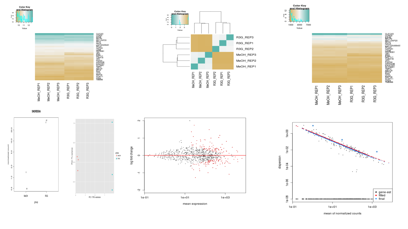
script would generate a tsv file (HTSeq summary), Images (summarizing sample properties, DE) and final .rdata for re running the analysis. User can modify the code htseq.r independent of bash script.
Images produced look like: