When biologists plot genes/SNPs of interest in a high density plot, highlighing genes/SNPs of interest is one of the main problems. Given below here is the easiest (probably crude) way to highlight genes/SNPs of interest. Please remember that this can be extended to any plot of user's choice. Logic is
Requirements:
Case study: User would like to know clinically significant variants per gene using clinvar vcf and highlight genes with highest variants.
Methods: 1) User creates a table with genes and clinical variants per gene in R
2) Highlight the genes with more than 1000/ 500 variants in two different examples.
Working example:
1) Navigate to the directory where the files are located (clinvar.vcf and clinvar.tab).
2) Print the lines in clinvar.tab.
command: wc -l clinvar.tab. Note down the number
3) Launch R/ Rstudio from the same directory. If R is launched from the else where, set the working directory to the directory where the files are located (using command setwd in R).
4) Import clinvar.tab file into R.
command: tab_clinvar=read.delim2("clinvar.tab")
5) Count the numer of imported entries
command: dim(tab_clinvar).
This should two values ( some thing like 121079 , 65). The first number gives the total number of entries and should match with that of clinvar.tab mentioned in step 2.
6) Please look at the column names (metadata) in the tab_clinvar object (data.frame).
command: colnames(tab_clinvar)
This will display all the columns (metadata for each variant) and should be around 65.Gene column would be GENEINFO. This would have Gene Symbol and corresponding ID together (but separated by full colon).
7) Subset the data to identify all the genes and variants per each gene and store it as a separate object. This would be used for the plot.
command: tab_gene=table(tab_clinvar$GENEINFO)
8) Look at the created table tab_gene.
command: dim(tab_gene); class(tab_gene)
This would display the entries (number of genes) in the table and the class (type) of the object, tab_gene in R, which would be table, in this case.
9) Convert the type of the object, tab_gene from class to data.frame.
command: tab_gene=as.data.frame(tab_gene)
10) Check again the numer of entries and type of the object.
command: dim(tab_gene); class(tab_gene).
Number displayed should be the same as those in step 8 and class should be data.frame, instead of table.
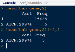
11) Look at the first two lines of object tab_gene. Please note that there would be an extra line with a large number. This should be removed before proceeding further. This extra line means that there are around 15689 without any genes being assigned to them i.e either they are unassigned or fall in intergenic /regulatory regions.
Commands:
head (tab_gene,2) #This would print first two lines
head (tab_gene,2)[-1,] # This would remove first row
tab_gene=tab_gene[-1,] # This would remove the first row of the object, tab_gene and saves it as tab_gene (same object but without first line)
head (tab_gene,2) # This would display updated object.
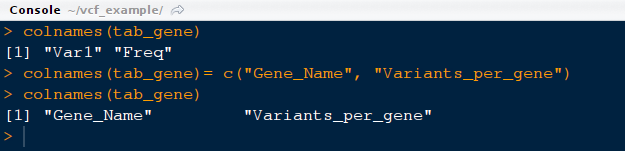
12) Please note that column names are not descriptive the contents. Let us change the name of the columns for better representation.
command: colnames(tab_gene)= c("Gene_Name", "Variants_per_gene")

13) Run some basic statistics to know about the number of variants per gene. For eg. maximum number of variants, average number of variants etc.
command: summary(tab_gene$Variants_per_gene)
This would give us the maximum number of variants observed for a gene, average number of variants per gene and most common variant number for most of the genes.
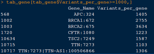
14) Let us look at the genes with more than 1000 clinical variants per gene.
command: tab_gene[tab_gene$Variants_per_gene>=1000,]. This should like this:
15) Let us store the list of genes with more than 1000 clinical variants per gene.
command:tab_gene_1000=tab_gene[tab_gene$Variants_per_gene>=1000,]
16) Like wise, let us store the list of genes with more than 500 clinical variants per gene.
command: tab_gene_500=tab_gene[tab_gene$Variants_per_gene>=500,]
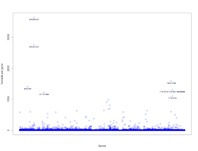
17) Let us plot number of total number variants per each gene. Numer of variants per gene on Y-axis and genes on X-axis. Let us not label tick marks on X-axis as the listing of ~11k gene names on X-axis would look messy.
command:
plot(tab_gene$Variants_per_gene, xlab="Genes", ylab="Variants per gene", pch=21, col="blue", xaxt="n")
(parameter: pch=21 means empty circles, xaxt = n means do not draw tick marks and tick labels)
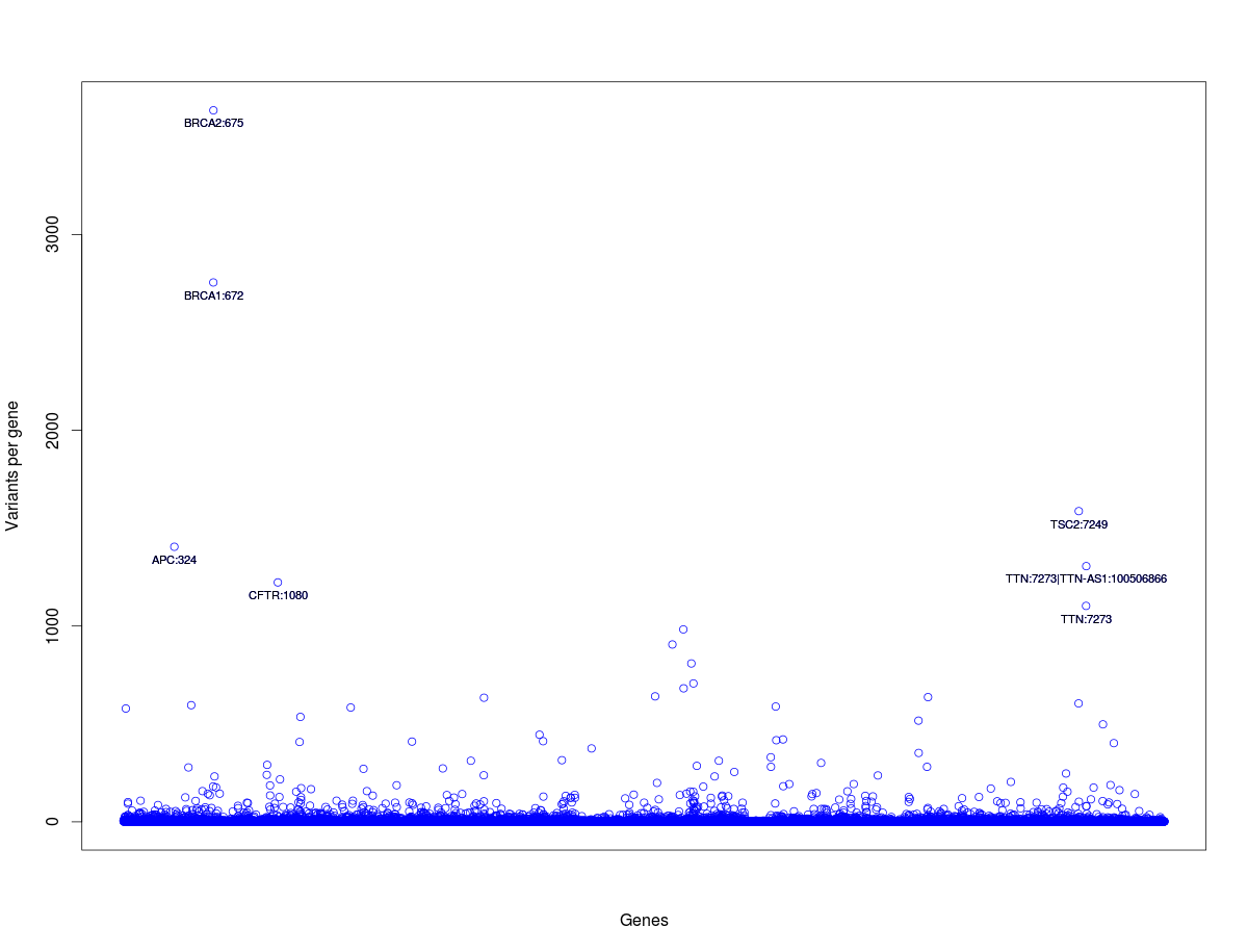
 13) Label the gene list with more than 1000 variants per gene.
command:text(x=rownames(tab_gene_1000), y=tab_gene_1000$Variants_per_gene, labels=tab_gene_1000$Gene_Name,cex=0.7, pos=1)
and should look like this:
 18) User can test the same code with genes with more than 500 variants with the list from step 16.
19) User can list the top 20 genes with highest number of variants
command: tab_gene_top20=head(tab_gene[order(-tab_gene$Variants_per_gene),],20)
20) Labeled top 20 genes will look following way

head(tab_clinvar) # Displays top lines of object
colnames(tab_clinvar) # Displays the column names (meta data) of clinvar data
tab_gene=table(tab_clinvar$GENEINFO) # stores the variant number per gene for all the genes
dim(tab_gene); class(tab_gene) # displays the dimensions and type of the object
head(tab_gene) # displays the first few lines of the object
tab_gene=as.data.frame(tab_gene) # converts the object as data.frame
dim(tab_gene); class(tab_gene) # displays the dimentions and type of the object
colnames(tab_gene) # Column names of the object are displayed
head(tab_gene,2) # first two lines of the object are printed
head(tab_gene,2)[-1,] # Removes first line of two lines printed above
tab_gene=tab_gene[-1,] # Removes the first line of the objest and stores the remainig object with the same name
head(tab_gene,2) # Displays first two lines of the object
colnames(tab_gene) # Displays the column names of the object
colnames(tab_gene)= c("Gene_Name", "Variants_per_gene") # changes the column names of the object
colnames(tab_gene) # displays the column names
summary(tab_gene$Variants_per_gene) # Displays basic summary of variants per gene
tab_gene[tab_gene$Variants_per_gene>=1000,] # Displays genes with more than 1000 variants per gene
tab_gene_1000=tab_gene[tab_gene$Variants_per_gene>=1000,] # stores the genes with more than 1000 variants per gene
tab_gene_1000 # displays the stored genes with more than 1000 variats per gene
tab_gene_500=tab_gene[tab_gene$Variants_per_gene>=500,] # stores the genes with more than 500 variants
tab_gene_500 # dispalys the stored genes with more than 500 variants
text(x=rownames(tab_gene_top20), y=tab_gene_top20$Variants_per_gene, labels=tab_gene_top20$Gene_Name,cex=0.7, pos=1) # labels the top 20 genes (please plot before running this code)
Please note that dplyr package, further simplifies summary of variants per gene.
For those, who is interested, my session info is:

- plot all the genes/SNPs in the genes of interest (main data)
- subset genes/snps that are of interest either by creating a list of genes (list in R/Bioc) or from the main data it self. (subset data)
- If it is user supplied list, then one needs to get the index and rest of the fields necessary to hightlight, from the main data. If it is later case, user can highlight as such without matching with main data. Example given below is the later case.
- highlight the subset data with custom commands.
Requirements:
- Example VCF file for parsing. Please follow the instructions below:
- Download the latest clinvar vcf file from NCBI ftp site. Current working link is : ftp://ftp.ncbi.nlm.nih.gov/pub/clinvar/vcf_GRCh38/clinvar.vcf.gz (file is around 5.1 MB)
- After downloading unzip the file.
command: gunzip clinvar.vcf. gz. This would create a vcf file of size 47 MB. - Convert the VCF file to tab separated file using vcflib program (https://github.com/ekg/vcflib) by runing the following command.
vcf2tsv clinvar.vcf > clinvar. tab. This would create a tab separated file of size 35 MB. (please note that vcf2tsv doesn't work on all vcfs. For eg. ENSEMBL-VEP output VCF can't be parsed in full with this command.)
Case study: User would like to know clinically significant variants per gene using clinvar vcf and highlight genes with highest variants.
Methods: 1) User creates a table with genes and clinical variants per gene in R
2) Highlight the genes with more than 1000/ 500 variants in two different examples.
Working example:
1) Navigate to the directory where the files are located (clinvar.vcf and clinvar.tab).
2) Print the lines in clinvar.tab.
command: wc -l clinvar.tab. Note down the number
3) Launch R/ Rstudio from the same directory. If R is launched from the else where, set the working directory to the directory where the files are located (using command setwd in R).
4) Import clinvar.tab file into R.
command: tab_clinvar=read.delim2("clinvar.tab")
5) Count the numer of imported entries
command: dim(tab_clinvar).
This should two values ( some thing like 121079 , 65). The first number gives the total number of entries and should match with that of clinvar.tab mentioned in step 2.
6) Please look at the column names (metadata) in the tab_clinvar object (data.frame).
command: colnames(tab_clinvar)
This will display all the columns (metadata for each variant) and should be around 65.Gene column would be GENEINFO. This would have Gene Symbol and corresponding ID together (but separated by full colon).
7) Subset the data to identify all the genes and variants per each gene and store it as a separate object. This would be used for the plot.
command: tab_gene=table(tab_clinvar$GENEINFO)
8) Look at the created table tab_gene.
command: dim(tab_gene); class(tab_gene)
This would display the entries (number of genes) in the table and the class (type) of the object, tab_gene in R, which would be table, in this case.
9) Convert the type of the object, tab_gene from class to data.frame.
command: tab_gene=as.data.frame(tab_gene)
10) Check again the numer of entries and type of the object.
command: dim(tab_gene); class(tab_gene).
Number displayed should be the same as those in step 8 and class should be data.frame, instead of table.
11) Look at the first two lines of object tab_gene. Please note that there would be an extra line with a large number. This should be removed before proceeding further. This extra line means that there are around 15689 without any genes being assigned to them i.e either they are unassigned or fall in intergenic /regulatory regions.

Commands:
head (tab_gene,2) #This would print first two lines
head (tab_gene,2)[-1,] # This would remove first row
tab_gene=tab_gene[-1,] # This would remove the first row of the object, tab_gene and saves it as tab_gene (same object but without first line)
head (tab_gene,2) # This would display updated object.
12) Please note that column names are not descriptive the contents. Let us change the name of the columns for better representation.
command: colnames(tab_gene)= c("Gene_Name", "Variants_per_gene")
13) Run some basic statistics to know about the number of variants per gene. For eg. maximum number of variants, average number of variants etc.
command: summary(tab_gene$Variants_per_gene)
This would give us the maximum number of variants observed for a gene, average number of variants per gene and most common variant number for most of the genes.
14) Let us look at the genes with more than 1000 clinical variants per gene.
command: tab_gene[tab_gene$Variants_per_gene>=1000,]. This should like this:

15) Let us store the list of genes with more than 1000 clinical variants per gene.
command:tab_gene_1000=tab_gene[tab_gene$Variants_per_gene>=1000,]
16) Like wise, let us store the list of genes with more than 500 clinical variants per gene.
command: tab_gene_500=tab_gene[tab_gene$Variants_per_gene>=500,]
17) Let us plot number of total number variants per each gene. Numer of variants per gene on Y-axis and genes on X-axis. Let us not label tick marks on X-axis as the listing of ~11k gene names on X-axis would look messy.
command:
plot(tab_gene$Variants_per_gene, xlab="Genes", ylab="Variants per gene", pch=21, col="blue", xaxt="n")
(parameter: pch=21 means empty circles, xaxt = n means do not draw tick marks and tick labels)

command:text(x=rownames(tab_gene_1000), y=tab_gene_1000$Variants_per_gene, labels=tab_gene_1000$Gene_Name,cex=0.7, pos=1)
and should look like this:
19) User can list the top 20 genes with highest number of variants
command: tab_gene_top20=head(tab_gene[order(-tab_gene$Variants_per_gene),],20)
20) Labeled top 20 genes will look following way

Entire code (assumption is that user knows how to save the images):
tab_clinvar=read.delim2("clinvar.tab") # imports clinvar variants table
dim(tab_clinvar) # Displays the dimentions of the objecthead(tab_clinvar) # Displays top lines of object
colnames(tab_clinvar) # Displays the column names (meta data) of clinvar data
tab_gene=table(tab_clinvar$GENEINFO) # stores the variant number per gene for all the genes
dim(tab_gene); class(tab_gene) # displays the dimensions and type of the object
head(tab_gene) # displays the first few lines of the object
tab_gene=as.data.frame(tab_gene) # converts the object as data.frame
dim(tab_gene); class(tab_gene) # displays the dimentions and type of the object
colnames(tab_gene) # Column names of the object are displayed
head(tab_gene,2) # first two lines of the object are printed
head(tab_gene,2)[-1,] # Removes first line of two lines printed above
tab_gene=tab_gene[-1,] # Removes the first line of the objest and stores the remainig object with the same name
head(tab_gene,2) # Displays first two lines of the object
colnames(tab_gene) # Displays the column names of the object
colnames(tab_gene)= c("Gene_Name", "Variants_per_gene") # changes the column names of the object
colnames(tab_gene) # displays the column names
summary(tab_gene$Variants_per_gene) # Displays basic summary of variants per gene
tab_gene[tab_gene$Variants_per_gene>=1000,] # Displays genes with more than 1000 variants per gene
tab_gene_1000=tab_gene[tab_gene$Variants_per_gene>=1000,] # stores the genes with more than 1000 variants per gene
tab_gene_1000 # displays the stored genes with more than 1000 variats per gene
tab_gene_500=tab_gene[tab_gene$Variants_per_gene>=500,] # stores the genes with more than 500 variants
tab_gene_500 # dispalys the stored genes with more than 500 variants
plot(tab_gene$Variants_per_gene, xlab="Genes", ylab="Variants per gene", pch=21, col="blue", xaxt="n") # plots the variants per gene with no ticks on x-axis
text(x=rownames(tab_gene_1000), y=tab_gene_1000$Variants_per_gene, labels=tab_gene_1000$Gene_Name,cex=0.7, pos=1) # adds the label to genes with more than 1000 variants
tab_gene_top20=head(tab_gene[order(-tab_gene$Variants_per_gene),],20) # stores top 20 genes in ascending order wrt variants per gene
Please note that dplyr package, further simplifies summary of variants per gene.
For those, who is interested, my session info is:
