RNAseq data analysis is a key tool in analyzing the expression trends between any two types (levels- eg. tumor, normal) under a given category ( factor - eg. disease). This can be applicable for more than 2 groups and more than 1 category based on analysis design. In this note, let us attempt a classical data analysis problem. We have NGS data for following and the data can be downloaded from here and the sample information (for eg. strand information RF is obtained from tutorials outlined here):
- 3 normal samples
- 3 tumor samples
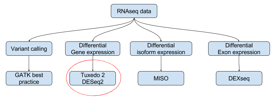
In general, RNAseq data can be used variant calling and differential expression (of genes, transcripts and exons).
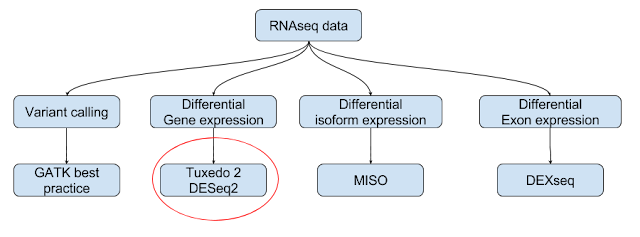 In this note, we will concentrate on Tuxedo protocol 2/ new tuxedo suite in this note. Work flow involves an aligner (HiSat2), an assembler (StringTie) and Analysis library (Ballgown- implemented in R). Tuxedo protocol 1 is covered else where in this blog.
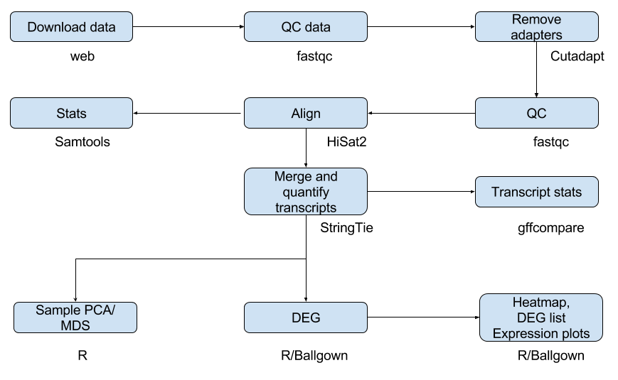
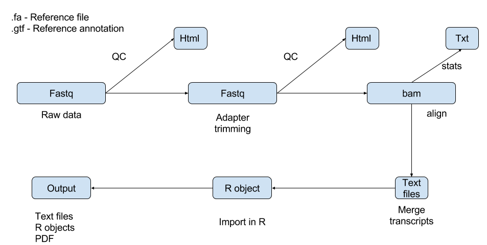
We will find the differentially expressed genes between two groups using HiSat2 work flows. HiSat2-StringTie-Ballgown workflow used in this note is explained below in two flow charts: one by tools used and another by input and output:
We will find the differentially expressed genes between two groups using HiSat2 work flows. HiSat2-StringTie-Ballgown workflow used in this note is explained below in two flow charts: one by tools used and another by input and output:
Work flow by tools used:
Work flow by input and output
We know that most of the steps in data analysis are individual steps and can be parallelized as there are many files to analyze. So let us use a tool called GNU-Parallel and it is very easy to use for this work flow.
Let us work step by step:
Note: User has a choice to organize the output. I prefer to store all my results tool wise i.e all the outputs from a fastqc are stored in a folder called fastqc with sample names appended to each output. However, HiSat2 workflow requires sample centric workflow i.e each sample has a folder and the output from all the tools for that sample is stored in sample folder. For eg. Sample A.fq will have a folder called Sample A and all the output from fastqc, hisat2, stringtie will be stored sample A folder.
I have used tool specific folder creation and user can modify the script as per user convenience. However, I switched to sample centric storage only at the end so that ballgown can load the data.
Extract reference sequence file
Reference files needed for RNAseq data analysis are reference fasta and reference annotation i.e transcript information (chromosomal coordinates of gene, transcript, exon in an organism). Reference sequence file is in fasta format (.fa) and annotation information is in .gtf format.
Sample reads we have align to chromosome 22. Hence we need to download chromosome 22 sequence and chromosome 22 annotation. Steps are:
- Download human genome sequence from UCSC (hg 38 is current version)
- Extract chromosome 22 sequence
$ faFilter -name=chr22 hg38.fa hg38.chr22.fa
Syntax for faFilter is chromosome name (chr22) inside reference fasta (hg38.fa) and the name to be saved (hg38.chr22.fa). You can download faFilter from Kentutils github page. Of course, there are several other tools to do this. But this is a tool with simple syntax.
$ wget -q https://genome.ucsc.edu/goldenpath/help/hg38.chrom.sizes -O - | grep -w chr22
output:
Build reference index files for HiSat2
$ mkdir fastqc
$ parallel --dry-run fastqc -q -o fastqc/ ::: raw_data/*.gz (This would pick up fastq.gz from raw_data directory and creates output files in a directory called fastqc (-o fastqc option and a dry run would be displayed on screen without actual execution).
$ parallel fastqc -q -o fastqc/ ::: raw_data/*.gz
Now, navigate to fastqc folder and execute mutliqc to summarize fastqc results.
$ multiqc . (. means current directory and multiqc automatically finds fastqc output and summarizes multiqc. This would create multiqc_report.html and mutqc_data. Results are summarized in multiqc_report.html and open it with a browser).
This would create a summary html file and open it with a browser
$ cd cutadapt
This would create fastqc otuput in the same directory. Now in this directory, we have trimmed sequences (12) and fastqc output. Now run multiqc in the same directory. This would pick up output files from both fastqc and cutadapt and summarizes both the results
$ multiqc .
$ mkdir hisat2
Validate reference sequence file
Now that we have made a new reference sequence file for chromosome 22 (hg38.chr22.fa), we need to validate it for it's size and number of bases. Run following commands.
$ seqkit stats hg38.chr22.fa
output:
file format type num_seqs sum_len min_len avg_len max_len
hg38.chr22.fa FASTA DNA 1 50,818,468 50,818,468 50,818,468 50,818,468
output:
chr22 50818468
Download seqkit from here. Seqkit outputs the type of the reference file which we know and size of the sequence (length). We have compared this length with that from UCSC, form chromosome 22. They match and this confirms that chromosome sequence we have is of chromosome 22.Build reference index files for HiSat2
Reference sequence file (.fa) needs to be indexed for alignment. HiSat2 creates both global and local index files for reference sequences. User can provide splice sites and reference transcript files for better indexing as this is a RNAseq data. Splice site calculation is done by script provided by same group. If you don't want to mess up the indexing, you can download the HiSat2 index files direct from here. They are huge as they are for entire genome. For partial reference sequences, it is better to index locally.
- Download gtf from UCSC or you can download it from here (hg38_ucsc_refseq_gtf.gz - 9MB ).
- Extract chromosome 22 annotation
$ zgrep -w chr22 hg38_ucsc_refseq_gtf.gz > chr22_hg38_ucsc_refseq_gtf.gz - Extract exons only from chromosome 22 gtf by using . This would be helpful in calculating splice sites
$ hisat2_extract_exons.py hg38_ucsc_refseq_chr22.gtf > hg38_ucsc_refseq_chr22_exons.gtf - Build splice sites
$ hisat2_extract_splice_sites.py hg38_ucsc_refseq_chr22.gtf > hg38_ucsc_refseq_chr22_splice.gtf - Index reference sequence file (chr22 fa), annotation (gtf) and calculated splice site file.
$ hisat2-build -p 6 --ss hg38_ucsc_refseq_chr22_splice.gtf --exon hg38_ucsc_refseq_chr22_exons.gtf hg38.chr22.fa hg38.chr22-p -- threads (6 here)
--ss -- splice site file
--exon -- exon file
hg38.chr22.fa -- reference sequence file
hg38.chr22 -- base name for index file
This would create 8 index files with .bt2 extension.
List raw files
Keep all sequence files (.fastq or .fq) in a directory called raw_data.
$mkdir raw_data
Sequence quality check using FastQC and MultiQC:
FastQC runs several sanity checks on each sequence and MultiQC summaizes output from FastQC. Since there are 6 files, there would be 6 outputs from FastQC and MultiQC summarizes all of them.
$ mkdir fastqc
$ parallel --dry-run fastqc -q -o fastqc/ ::: raw_data/*.gz (This would pick up fastq.gz from raw_data directory and creates output files in a directory called fastqc (-o fastqc option and a dry run would be displayed on screen without actual execution).
$ parallel fastqc -q -o fastqc/ ::: raw_data/*.gz
Now, navigate to fastqc folder and execute mutliqc to summarize fastqc results.
$ multiqc . (. means current directory and multiqc automatically finds fastqc output and summarizes multiqc. This would create multiqc_report.html and mutqc_data. Results are summarized in multiqc_report.html and open it with a browser).
If you look at the raw data quality, you would observe that there is Illumina universal adapter contamination and other issues. Other issues such as low quality and sequence duplication at the start of the sequence are very common to RNAseq and can be neglected. Let us remove the adapter sequences using a tool called cutadapt.
Remove adapter sequences
Adapter sequences can be removed using cutadapt and the command is given below. This would remove adapters and saves trimmed sequences in a different folder called cutadapt.
$ mkdir cutadapt
$ ls raw_data/*.gz| sed 's/r[1-2].fastq.gz$//' | parallel 'cutadapt -a AGATCGGAAGAGCACACGTCTGAACTCCAGTCAC -A AGATCGGAAGAGCGTCGTGTAGGGAAAGAGTGTAGATCTCGGTGGTCGCCGTATCATT -o ./cutadapt/{/.}r1_cutadapt.fastq.gz -p ./cutadapt/{/.}r2_cutadapt.fastq.gz {}r1.fastq.gz {}r2.fastq.gz &> ./cutadapt/{/.}cutadapt.log'
$ ls raw_data/*.gz| sed 's/r[1-2].fastq.gz$//' | parallel 'cutadapt -a AGATCGGAAGAGCACACGTCTGAACTCCAGTCAC -A AGATCGGAAGAGCGTCGTGTAGGGAAAGAGTGTAGATCTCGGTGGTCGCCGTATCATT -o ./cutadapt/{/.}r1_cutadapt.fastq.gz -p ./cutadapt/{/.}r2_cutadapt.fastq.gz {}r1.fastq.gz {}r2.fastq.gz &> ./cutadapt/{/.}cutadapt.log'
$ ls raw_data/*.gz - lists all gz files in raw_data folder
$ sed 's/r[1-2].fastq.gz$//' - Sed would remove extension (r1.fastq.gz and r2.fastq.gz) from all the files as this would be used as regular expression (common pattern) later
$ sed 's/r[1-2].fastq.gz$//' - Sed would remove extension (r1.fastq.gz and r2.fastq.gz) from all the files as this would be used as regular expression (common pattern) later
Rest of the the command would store ouput in cutadapt folder and log files would be stored as .log files in cutadapt directory. These log files will have all kinds of information such as sequences removed etc. Parallel{/.} would remove file path and file extension.
Summarize Cutadapt results with MultiQC
Navigate to cutadapt directory and execute multiqc inside it.
$ cd cutadapt
$ multiqc .
$ multiqc .
This would create a summary html file and open it with a browser
Rerun fastQC on trimmed sequences
$ cd cutadapt
$ parallel fastqc -q ::: *.gz
This would create fastqc otuput in the same directory. Now in this directory, we have trimmed sequences (12) and fastqc output. Now run multiqc in the same directory. This would pick up output files from both fastqc and cutadapt and summarizes both the results
$ multiqc .
Align trimmed sequences
Now important part of the analysis. Let us align the sequences with hisat2. We already created reference index files and we trimmed sequence files. Let us align the sequences to reference and use it's annotations. For this let us created a folder called hisat2 and put all the output there.
$ mkdir hisat2
$ find cutadapt/*.fastq.gz | xargs basename -a | sed 's/_r[1-2].*fastq.gz$//' |uniq | parallel --progress 'hisat2 --rg-id={} --rg SM:{} --rg PL:ILLUMINA -x ../../reference/hg38/hg38.chr22 --dta --rna-strandness RF -1 cutadapt/{}_r1_cutadapt.fastq.gz -2 cutadapt/{}_r2_cutadapt.fastq.gz -S ./hisat2/{}.cutadapt.sam &> ./hisat2/{}.hisat.log'
$ find cutadapt/*.fastq.gz -- find fastq.gz files in cutadapt directory
$ xargs basename -a -- remove file paths
$ sed 's/_r[1-2].*fastq.gz$//' -- remove _r1.fastq.gz and _r2.fastq.gz from file names which can be used as pattern later on
$ uniq - display only unique names
$ rg-id = read group id. We are supplying a common name. For eg. hcc1395_normal_rep1_r1_cutadapt.fastq.gz and hcc1395_normal_rep1_r2_cutadapt.fastq.gz will have hcc1395_normal_rep1 as group ID
$ rg-sm = read group sample name same as above
$ rg-PL = Platform (Illumina here)
-x = basename of index (read above for basename)
--dta - report alignments for downstream analysis (stringtie)
--rna-strandess = RF. This information is obtained from the site mentioned above
Above command displays the progress and stores the aligned files in HiSat2 directory. Since this is a paired end sequencing, we have one sam file for two fastq sequences (R1 and R2). Hence there are 6 sam files (3 for normal and 3 for tumor). Log files are also stored in hisat2 directory. If there are any issues, look into log files.
$ find hisat2/*.sam | parallel 'samtools view -bh {} | samtools sort - -o {.}.bam; samtools index {.}.bam'
Now that bam files are ready, we can do two things:
- merge bams to corresponding groups. For eg. all normal bams into one final bam and all tumor bams into one final tumor bam.
- Treat each bam separate till last. This is what i prefer.
Let us do both. Let us merge the bam files into corresponding final group bams. But grouped bams will not be used in downstream analysis as the code used for individual bams can be applied to grouped bam.
$ find cutadapt/*.fastq.gz -- find fastq.gz files in cutadapt directory
$ xargs basename -a -- remove file paths
$ sed 's/_r[1-2].*fastq.gz$//' -- remove _r1.fastq.gz and _r2.fastq.gz from file names which can be used as pattern later on
$ uniq - display only unique names
$ rg-id = read group id. We are supplying a common name. For eg. hcc1395_normal_rep1_r1_cutadapt.fastq.gz and hcc1395_normal_rep1_r2_cutadapt.fastq.gz will have hcc1395_normal_rep1 as group ID
$ rg-sm = read group sample name same as above
$ rg-PL = Platform (Illumina here)
-x = basename of index (read above for basename)
--dta - report alignments for downstream analysis (stringtie)
--rna-strandess = RF. This information is obtained from the site mentioned above
Above command displays the progress and stores the aligned files in HiSat2 directory. Since this is a paired end sequencing, we have one sam file for two fastq sequences (R1 and R2). Hence there are 6 sam files (3 for normal and 3 for tumor). Log files are also stored in hisat2 directory. If there are any issues, look into log files.
Convert sam to bam, sort and index bam files
Now sam files are in hisat2 directory and we need to convert them to bam file, index each bam file and then index them.
Now that bam files are ready, we can do two things:
- merge bams to corresponding groups. For eg. all normal bams into one final bam and all tumor bams into one final tumor bam.
- Treat each bam separate till last. This is what i prefer.
Let us do both. Let us merge the bam files into corresponding final group bams. But grouped bams will not be used in downstream analysis as the code used for individual bams can be applied to grouped bam.
Bam file statistics
$ mkdir bamstats
$ find hisat2/hcc*.bam | xargs basename -a | parallel 'samtools flagstat ./hisat2/{} > ./bamstats/{}.stats'
$ find hisat2/hcc*.bam | xargs basename -a | parallel 'samtools flagstat ./hisat2/{} > ./bamstats/{}.stats'
This would create one statistics file per bam file in hisat2 directory and bam files should start with hcc.
Merge bams
As I mentioned above, one can merge all normal bams into one single normal bam and all tumor bams into one tumor bam.
Merge all normal bams to one single normal bam:
$ bamtools merge -in ./hisat2/hcc1395_normal_rep1.cutadapt.bam -in ./hisat2/hcc1395_normal_rep2.cutadapt.bam -in ./hisat2/hcc1395_normal_rep3.cutadapt.bam -out ./hisat2/normal.bam
Merge all tumor bams to one single tumor bam:
$ bamtools merge -in ./hisat2/hcc1395_tumor_rep1.cutadapt.bam -in ./hisat2/hcc1395_tumor_rep2.cutadapt.bam -in ../hisat2/hcc1395_tumor_rep3.cutadapt.bam -out tumor.bam
$ bamtools merge -in ./hisat2/hcc1395_tumor_rep1.cutadapt.bam -in ./hisat2/hcc1395_tumor_rep2.cutadapt.bam -in ../hisat2/hcc1395_tumor_rep3.cutadapt.bam -out tumor.bam
Now you will have two additional bam files in hisat2 directory, normal and tumor bam. However, let us run rest of the analysis on individual bams and then use ballgown package for differential expression. Please note that the same script can be used for combined bams as well.
Extract transcript information from bam (as transcripts, introns, exons) and corresponding quantitative information. StringTie can build transcripts, exons and intron information (as transcript.gtf for each sample) along with quantitative information. In this step, let us create a directory by name "stringtie" and 6 subdirectories so that stringtie creates all the necessary files. This is because stringtie creates several files by common name (such as i.tab, e.tab etc). Once we do this, we can load the files in R as ballgown looks for a directory structure, for loading input files. In addition, tool provided by hisat2 (
stringtie_expression_matrix.pl) needs directory structure.
Using StringTie, we are going to do many things:
1) Create transcript, exon, intron files (transcripts.gtf, e.tab, i.tab etc) one for each bam file using StringTie
2) Merge all transcripts (merged transcript file for all the samples)
3) Extract FPKM, TPM and Coverage file individually for all samples. This can be used for further analysis, if user wants to.
4) Create necessary files and load them into R via Ballgown library.
Create transcripts using StringTie
$ mkdir stringtie
$ ls hisat2/*hcc*.bam | xargs basename -a | cut -f1 -d "." | parallel mkdir stringtie/{}
$ ls -d stringtie/* | parallel echo {/} | parallel --progress 'stringtie -G ../../reference/hg38/hg38_ucsc_refseq_chr22.gtf --rf -e -B -o ./stringtie/{}/transcripts.gtf -A ./stringtie/{}/gene_abundances.tsv -C ./stringtie/{}/cov_ref.gtf --rf ./hisat2/{}.cutadapt.bam &> ./stringtie/{}/stringtie.log'
2nd command would create 6 directories under stringtie directory and the names will match those bam files from hisat2.
3rd command would create output from StringTie in each sample directory. Each sample directory will have 9 files including log. If every thing goes well, log files would be empty. In above command we created, output files necessary for ballgown, coverage file, abundance file and transcript file.
Merge all the transcripts
Now, let us merge all the transcripts.
$ cd stringtie
$ find | grep transc | xargs stringtie --merge -G /home/suresh/reference/hg38/hg38_ucsc_refseq_chr22.gtf -o merge_transcripts.gtf
This would create merged transcripts.gtf file for further analysis.
Above command would find transcript gtf in all the subdirectories of stringtie directory, but skips those files with merge string in it. gffcompare will compare transcripts.gtf in each subdirectory and creates several files post comparison. Basename of all the files created by gffcompare will have strcmp to them. You would need to look at strcmp.stats file for overall matching.
Compare output transcript (transcript.gtf) with reference gtf
Once transcript map for each sample. We want to compare this transcript map with reference transcript information (reference gtf).
$ cd stringtie
$ find
|grep -P trans.*.gtf$ | grep -v merge | parallel --progress
gffcompare -G -r ~/reference/hg38/hg38_ucsc_refseq_chr22.gtf -o
{//}/strcmp {}
Count and extract FPKM, Coverage, TPM
Extract and count FPKMs for all the samples:
$ cd stringtie
$ perl ../stringtie_expression_matrix.pl --expression_metric=FPKM --result_dirs='hcc1395_normal_rep1,hcc1395_normal_rep2,hcc1395_normal_rep3,hcc1395_tumor_rep1,hcc1395_tumor_rep2,hcc1395_tumor_rep3' --transcript_matrix_file=transcript_fpkm_all_samples.tsv --gene_matrix_file=gene_fpkm_all_samples.tsv
(note: Download stringtie_expression_matrix.pl and keep it in analysis folder. Stringtie folder on my machine is a subfolder of analysis which is why in command line, it is kept above stringtie folder. Be careful with double -- while copying)
Extract and count coverage for all samples
$ cd stringtie
$ perl ../stringtie_expression_matrix.pl --expression=coverage --result_dirs='hcc1395_normal_rep1,hcc1395_normal_rep2,hcc1395_normal_rep3,hcc1395_tumor_rep1,hcc1395_tumor_rep2,hcc1395_tumor_rep3' --transcript_matrix_file=transcript_coverage_all_samples.tsv --gene_matrix_file=gene_coverage_all_samples.tsv
$ perl ../stringtie_expression_matrix.pl --expression=coverage --result_dirs='hcc1395_normal_rep1,hcc1395_normal_rep2,hcc1395_normal_rep3,hcc1395_tumor_rep1,hcc1395_tumor_rep2,hcc1395_tumor_rep3' --transcript_matrix_file=transcript_coverage_all_samples.tsv --gene_matrix_file=gene_coverage_all_samples.tsv
Extract and count TPMs for all samples
$ cd stringtie
$ perl ../stringtie_expression_matrix.pl --expression_metric=TPM --result_dirs='hcc1395_normal_rep1,hcc1395_normal_rep2,hcc1395_normal_rep3,hcc1395_tumor_rep1,hcc1395_tumor_rep2,hcc1395_tumor_rep3' --transcript_matrix_file=transcript_samples.tsv --gene_matrix_file=gene_tpms_all_samples.tsv
Now we are done with Sequence quality check, sequence trimming, alignment and post alignment. Let us do analysis with Ballgown package in R.
This page is already long. Let me create a new page for ballgown analysis and you can view it here.